| Title: | Add a Scale Bar to 'OpenStreetMap' Plots |
| Version: | 0.5.23 |
| Date: | 2025-09-30 |
| Maintainer: | Berry Boessenkool <berry-b@gmx.de> |
| Description: | Functionality to handle and project lat-long coordinates, easily download background maps and add a correct scale bar to 'OpenStreetMap' plots in any map projection. |
| Imports: | OpenStreetMap, berryFunctions (≥ 1.15.0), sf, pbapply |
| URL: | https://github.com/brry/OSMscale |
| License: | GPL-2 | GPL-3 [expanded from: GPL (≥ 2)] |
| Encoding: | UTF-8 |
| RoxygenNote: | 7.3.3 |
| Suggests: | testthat |
| BugReports: | https://github.com/brry/OSMscale/issues |
| NeedsCompilation: | no |
| Packaged: | 2025-09-30 08:26:02 UTC; berry |
| Author: | Berry Boessenkool [aut, cre] |
| Repository: | CRAN |
| Date/Publication: | 2025-09-30 08:50:19 UTC |
Add a Scalebar to OpenStreetMap Plots
Description
Functionality to handle and project lat-long coordinates, easily download background maps and add a correct scale bar to 'OpenStreetMap' plots in any map projection. There are some other spatially related miscellaneous functions as well.
Note
Get the most recent code updates at https://github.com/brry/OSMscale
Author(s)
Berry Boessenkool, berry-b@gmx.de, June 2016
See Also
scaleBar, pointsMap, projectPoints,
mapmisc article at https://journal.r-project.org/archive/2016-1/brown.pdf
Examples
if(FALSE){ # Not tested on CRAN to avoid download time
d <- read.table(sep=",", header=TRUE, text=
"lat, long
55.685143, 12.580008
52.514464, 13.350137
50.106452, 14.419989
48.847003, 2.337213
51.505364, -0.164752")

# zoom set to 3 to speed up tests. automatic zoom determination is better.
map <- pointsMap(lat, long, data=d, type="esri",
                 proj=putm(d$long), scale=FALSE, zoom=3, pch=16, col=2)
scaleBar(map, abslen=500, y=0.8, cex=0.8)
lines(projectPoints(d$lat, d$long), col="blue", lwd=2)
}
GPS recorded bike track
Description
My daily bike route, recorded with the app OSMtracker on my Samsung Galaxy S5
Format
'data.frame': 254 obs. of 4 variables:
$ lon : num 13 13 13 13 13 ...
$ lat : num 52.4 52.4 52.4 52.4 52.4 ...
$ time: POSIXct, format: "2016-05-18 07:53:22" "2016-05-18 07:53:23" ...
$ ele : num 66 66 66 67 67 67 68 69 69 69 ....
Source
GPS track export from OSMtracker App
Examples
data(biketrack)
plot(biketrack[,1:2])
# see equidistPoints
lat-long coordinate check
Description
check lat-long coordinates for plausibility
Usage
checkLL(lat, long, data, fun = stop, quiet = FALSE, ...)
Arguments
lat, long |
Latitude (North/South) and longitude (East/West) coordinates in decimal degrees |
data |
Optional: data.frame with the columns |
fun |
One of the functions |
quiet |
Logical: suppress non-df warning in |
... |
Further arguments passed to |
Value
Invisible T/F vector showing which of the coordinates is violated in the order: minlat, maxlat, minlong, maxlong. Only returned if check is passed or fun != stop
Author(s)
Berry Boessenkool, berry-b@gmx.de, Aug 2016
See Also
pointsMap, putm,
berryFunctions::checkFile
Examples
checkLL(lat=52, long=130)
checkLL(130, 52, fun=message)
checkLL(85:95, 0, fun=message)

d <- data.frame(x=0, y=0)
checkLL(y,x, d)

# informative errors:
library("berryFunctions")
is.error(   checkLL(85:95, 0, fun="message"),  tell=TRUE)
is.error(   checkLL(170,35),  tell=TRUE)

mustfail <- function(expr) stopifnot(berryFunctions::is.error(expr))
mustfail( checkLL(100)         )
mustfail( checkLL(100, 200)    )
mustfail( checkLL(-100, 200)   )
mustfail( checkLL(90.000001, 0)   )
decimal degree coordinate conversion
Description
Convert latitude-longitude coordinates between decimal representation and degree-minute-second notation
Usage
degree(
  lat,
  long,
  data,
  todms = !is.character(lat),
  digits = 1,
  drop = FALSE,
  quiet = FALSE
)
Arguments
lat, long |
Latitude (North/South) and longitude (East/West) coordinates in decimal degrees |
data |
Optional: data.frame with the columns |
todms |
Logical specifying direction of conversion. If FALSE, converts to decimal degree notation, splitting coordinates at the symbols for degree, minute and second (\U00B0, ', "). DEFAULT: !is.character(lat) |
digits |
Number of digits the seconds are |
drop |
Drop to lowest dimension? DEFAULT: FALSE |
quiet |
Logical: suppress non-df warning in |
Value
data.frame with x and y as character strings or numerical values, depending on conversion direction
Author(s)
Berry Boessenkool, berry-b@gmx.de, Aug 2016
See Also
earthDist, projectPoints for geographical reprojection
Examples
# DECIMAL to DMS notation: --------------------------------------------------
degree(52.366360, 13.024181)
degree(c(52.366360, -32.599203), c(13.024181,-55.809601))
degree(52.366360, 13.024181, drop=TRUE) # vector
degree(47.001, -13.325731, digits=5)

# Use table with values instead of single vectors:
d <- read.table(header=TRUE, sep=",", text="
lat, long
 52.366360,  13.024181
-32.599203, -55.809601")
degree(lat, long, data=d)

# DMS to DECIMAL notation: --------------------------------------------------
# You can use the degree symbol and escaped quotation mark (\") as well.
degree("52'21'58.9'N", "13'1'27.1'E")
print(degree("52'21'58.9'N", "13'1'27.1'E"), digits=15)

d2 <- read.table(header=TRUE, stringsAsFactors=FALSE, text="
lat long
52'21'58.9'N 13'01'27.1'E
32'35'57.1'S 55'48'34.6'W") # columns cannot be comma-separated!
degree(lat, long, data=d2)

# Rounding error checks: ----------------------------------------------------
oo <- options(digits=15)
d
degree(lat, long, data=degree(lat, long, d))
degree(lat, long, data=degree(lat, long, d, digits=3))
options(oo)
stopifnot(all(degree(lat,long,data=degree(lat,long,d, digits=3))==d))
distance between lat-long coordinates
Description
Great-circle distance between points at lat-long coordinates.
(The shortest distance over the earth's surface).
The distance of all the entries is computed relative to the ith one.
Usage
earthDist(lat, long, data, r = 6371, i = 1L, along = FALSE, quiet = FALSE)
Arguments
lat, long |
Latitude (North/South) and longitude (East/West) coordinates in decimal degrees |
data |
Optional: data.frame with the columns |
r |
radius of the earth. Could be given in miles. DEFAULT: 6371 (km) |
i |
Integer: Index element against which all coordinate pairs are computed. DEFAULT: 1 |
along |
Logical: Should distances be computed along vector of points?
If TRUE, |
quiet |
Logical: suppress non-df warning in |
Value
Vector with distance(s) in km (or units of r, if r is changed)
Author(s)
Berry Boessenkool, berry-b@gmx.de, Aug 2016 + Jan 2017. Angle formula from Diercke Weltatlas 1996, Page 245
See Also
maxEarthDist, degree for pre-formatting,
http://www.movable-type.co.uk/scripts/latlong.html
Examples
d <- read.table(header=TRUE, sep=",", text="
lat, long
52.514687,  13.350012   # Berlin
51.503162,  -0.131082   # London
35.685024, 139.753365") # Tokio
earthDist(lat, long, d)      # from Berlin to L and T: 928 and 8922 km
earthDist(lat, long, d, i=2) # from London to B and T: 928 and 9562 km

# slightly different with other formulas:
# install.packages("geosphere")
# geosphere::distHaversine(as.matrix(d[1,2:1]), as.matrix(d[2,2:1])) / 1000

# Distance along vector of points:
d <- data.frame(lat=21:50, long=1:30)
pointsMap(lat,long,d, zoom=2, proj=putm(1:30) )
along1 <- earthDist(lat,long,d, along=TRUE)
along2 <- c(0, sapply(2:nrow(d), function(i) earthDist(lat,long,data=d[i-1:0,])[2]))
along1-along2 # all zero, but second version is MUCH slower for large datasets


# compare with UTM distance
set.seed(42)
d <- data.frame(lat=runif(100, 47,54), long=runif(100, 6, 15))
d2 <- projectPoints(d$lat, d$long)
d_utm <- berryFunctions::distance(d2$x[-1],d2$y[-1], d2$x[1],d2$y[1])/1000
d_earth <- earthDist(lat,long, d)[-1]
plot(d_utm, d_earth) # distances in km
hist(d_utm-d_earth) # UTM distance slightly larger than earth distance
plot(d_earth, d_utm-d_earth) # correlates with distance
berryFunctions::colPoints(d2$x[-1], d2$y[-1], d_utm-d_earth, add=FALSE)
points(d2$x[1],d2$y[1], pch=3, cex=2, lwd=2)
Evenly spaced points along path
Description
Compute waypoints with equal distance to each other along a (curved) path or track given by coordinates
Usage
equidistPoints(x, y, z, data, n, nint = 30, mid = FALSE, quiet = FALSE, ...)
Arguments
x, y, z |
Vectors with coordinates. z is optional and can be left empty |
data |
Optional: data.frame with the column names as given by x,y (and z) |
n |
Number of segments to create along the path (=number of points-1) |
nint |
Number of points to interpolate between original coordinates (with |
mid |
Logical: Should centers of segments be returned instead of their ends? |
quiet |
Logical: suppress non-df warning in |
... |
Further arguments passed to |
Value
Dataframe with the coordinates of the final points. ATTENTION: The columns are named x,y,z, not with the original names from the function call.
Author(s)
Berry Boessenkool, berry-b@gmx.de, May 2016
See Also
berryFunctions::distance and berryFunctions::approx2
Examples
library(berryFunctions) # distance, colPoints etc
x <- c(2.7, 5, 7.8, 10.8, 13.7, 15.8, 17.4, 17.7, 16.2, 15.8, 15.1, 13.1, 9.3, 4.8, 6.8, 12.2)
y <- c(2.3, 2.1, 2.6, 3.3, 3.7, 4.7, 7.6, 11.7, 12.4, 12.3, 12.3, 12.3, 12, 12.1, 17.5, 19.6)
eP <- equidistPoints(x,y, n=10) ; eP
plot(x,y, type="o", pch=4)
points(equidistPoints(x,y, n=10), col=4, pch=16)
points(equidistPoints(x,y, n=10, nint=1), col=2) # from original point set
round(distance(eP$x, eP$y), 2) # the 2.69 instead of 4.50 is in the sharp curve
# These points are quidistant along the original track

plot(x,y, type="o", pch=16, col=2)
round(sort(distance(x,y)), 2)
xn <- equidistPoints(x,y, n=10)$x
yn <- equidistPoints(x,y, n=10)$y
lines(xn,yn, type="o", pch=16)
round(sort(distance(xn,yn)), 2)
for(i in 1:8)
{
xn <- equidistPoints(xn,yn, n=10)$x
yn <- equidistPoints(xn,yn, n=10)$y
lines(xn,yn, type="o", pch=16)
print(round(sort(distance(xn,yn)), 2))
} # We may recursively get closer to equidistant along track _and_ air,
# but never actually reach it.

# Real dataset:
data(biketrack)
colPoints("lon","lat","ele",data=biketrack, add=FALSE,asp=1,pch=4,lines=TRUE)
points(equidistPoints(lon, lat, data=biketrack, n=25), pch=3, lwd=3, col=2)
bt2 <- equidistPoints(lon, lat, ele, data=biketrack, n=25)
bt2$dist <- distance(bt2$x, bt2$y)*1000
colPoints("x", "y", "z", data=bt2, legend=FALSE)
# in curves, crow-distance is shorter sometimes
plot(lat~lon, data=biketrack, asp=1, type="l")
colPoints("x","y","dist",data=bt2, Range=c(2.5,4),add=TRUE,asp=1,pch=3,lwd=5)
lines(lat~lon, data=biketrack)
Compare map tiles
Description
Compare map tiles
Usage
mapComp(
  lat,
  long,
  data,
  types = NA,
  progress = TRUE,
  file = "mapComp.pdf",
  overwrite = FALSE,
  pargs = NULL,
  quiet = FALSE,
  ...
)
Arguments
lat, long, data |
Coordinates as in |
types |
Character string vector, types for
|
progress |
Display progress bar? DEFAULT: TRUE |
file |
PDF filename. Will not be overwritten unless |
overwrite |
Overwrite pdf file? DEFAULT: FALSE |
pargs |
List of arguments passed to |
quiet |
Logical: suppress non-df warning in |
... |
Further arguments passed to |
Value
List of maps, writes to a pdf
Author(s)
Berry Boessenkool, berry-b@gmx.de, Jul 2017
See Also
Examples
## Not run:  # Exclude from CRAN checks because of download time
maps <- mapComp(c(52.39,52.46), c(12.99,13.06),
                pargs=list(width=8.27, height=11.96), overwrite=TRUE)

# still need to suppress output to console:
# https://stackoverflow.com/questions/45041762/suppress-rjava-error-output-in-console

unlink("mapComp.pdf")

## End(Not run)
maximum distance between set of points
Description
Maximum great-circle distance between points at lat-long coordinates. This is not computationally efficient. For large datasets, consider pages like https://stackoverflow.com/a/16870359.
Usage
maxEarthDist(
  lat,
  long,
  data,
  r = 6371,
  fun = max,
  each = TRUE,
  quiet = FALSE,
  ...
)
Arguments
lat, long, data |
Coordinates for |
r |
Earth Radius for |
fun |
Function to be applied. DEFAULT: |
each |
Logical: give max dist to all other points for each point separately?
If FALSE, will return the maximum of the complete distance matrix,
as if |
quiet |
Logical: suppress non-df warning in |
... |
Further arguments passed to fun, like na.rm=TRUE |
Value
Single number
Author(s)
Berry Boessenkool, berry-b@gmx.de, Jan 2017
See Also
Examples
d <- read.table(header=TRUE, text="
    x     y
14.9 53.73
1.12 53.12
6.55 58.13
7.71 71.44
")

plot(d, asp=1, pch=as.character(1:4), xlab="lon", ylab="lat")
for(i in 1:4) segments(d$x[-i], d$y[-i], d$x[i], d$y[i], col=2)
text(x=c(7,10,11), y=c(53,56,64), round(earthDist(y,x,d    )[-1]),  col=2)
text(x=c(4,4),     y=c(56,61),    round(earthDist(y,x,d,i=2)[3:4]), col=2)
text(x=7,          y=64,          round(earthDist(y,x,d,i=4)[3]),   col=2)

round(  earthDist(y,x,d, i=2)   )
round(  earthDist(y,x,d, i=3)   )

round(  maxEarthDist(y,x,d)              )
round(  maxEarthDist(y,x,d, each=FALSE)  )
round(  maxEarthDist(y,x,d, fun=min)     )

maxEarthDist(y,x, d[1:2,] )
Get map for lat-long points
Description
Download and plot map with the extend of a dataset with lat-long coordinates.
Usage
pointsMap(
  lat,
  long,
  data,
  ext = 0.07,
  fx = 0.05,
  fy = fx,
  type = "osm",
  zoom = NULL,
  minNumTiles = 9L,
  mergeTiles = TRUE,
  map = NULL,
  proj = NA,
  plot = TRUE,
  mar = c(0, 0, 0, 0),
  add = FALSE,
  scale = TRUE,
  quiet = FALSE,
  pch = 3,
  col = "red",
  cex = 1,
  bg = NA,
  pargs = NULL,
  titleargs = NULL,
  ...
)
Arguments
lat, long |
Latitude (North/South) and longitude (East/West) coordinates in decimal degrees |
data |
Optional: data.frame with the columns |
ext |
Extension added in each direction if a single coordinate is given. DEFAULT: 0.07 |
fx, fy |
Extend factors (additional map space around actual points)
passed to custom version of |
type |
Tile server in |
zoom, minNumTiles, mergeTiles |
Arguments passed to |
map |
Optional map object. If given, it is not downloaded again. Useful to project maps in a second step. DEFAULT: NULL |
proj |
If you want to reproject the map (Consumes some extra time), the
proj4 character string or CRS object to project to, e.g. |
plot |
Logical: Should map be plotted and points added? Plotting happens with
|
mar |
Margins to be set first (and left unchanged). DEFAULT: c(0,0,0,0) |
add |
Logical: add points to existing map? DEFAULT: FALSE |
scale |
Logical: should |
quiet |
Logical: suppress progress messages and non-df warning in
|
pch, col, cex, bg |
Arguments passed to |
pargs |
List of arguments passed to |
titleargs |
List of arguments passed to |
... |
Further arguments passed to |
Value
Map returned by OpenStreetMap::openmap
Author(s)
Berry Boessenkool, berry-b@gmx.de, Jun 2016
See Also
projectPoints, OpenStreetMap::openmap
Examples
if(interactive()){
d <- read.table(sep=",", header=TRUE, text=
"lat, long # could e.g. be copied from googleMaps, rightclick on What's here?
43.221028, -123.382998
43.215348, -123.353804
43.227785, -123.368694
43.232649, -123.355895")

map <- pointsMap(lat, long, data=d)
if(!is.character(map)){ # failed maps return a character string
axis(1, line=-2); axis(2, line=-2) # in whatever unit
map_utm <- pointsMap(lat, long, d, map=map, proj=putm(d$long))
axis(1, line=-2); axis(2, line=-2) # now in meters
projectPoints(d$lat, d$long)
scaleBar(map_utm, x=0.2, y=0.8, unit="mi", type="line", col="red", length=0.25)
pointsMap(lat, long, d[1:2,], map=map_utm, add=TRUE, col="red", pch=3, pargs=list(lwd=3))
}

d <- data.frame(long=c(12.95, 12.98, 13.22, 13.11), lat=c(52.40,52.52, 52.36, 52.45))
map <- pointsMap(lat,long,d, type="bing") # aerial map
}
CRS of various PROJ.4 projections
Description
coordinate reference system (CRS) Object for several proj4 character strings.
posm and pll are taken directly from
OpenStreetMap::osm and
longlat.
pmap gets the projection string from map objects as returned by pointsMap.
Usage
putm(long, zone = mean(long, na.rm = TRUE)%/%6 + 31)

posm()

pll()

pmap(map)
Arguments
long |
Vector of decimal longitude coordinates (East/West values).
Not needed of |
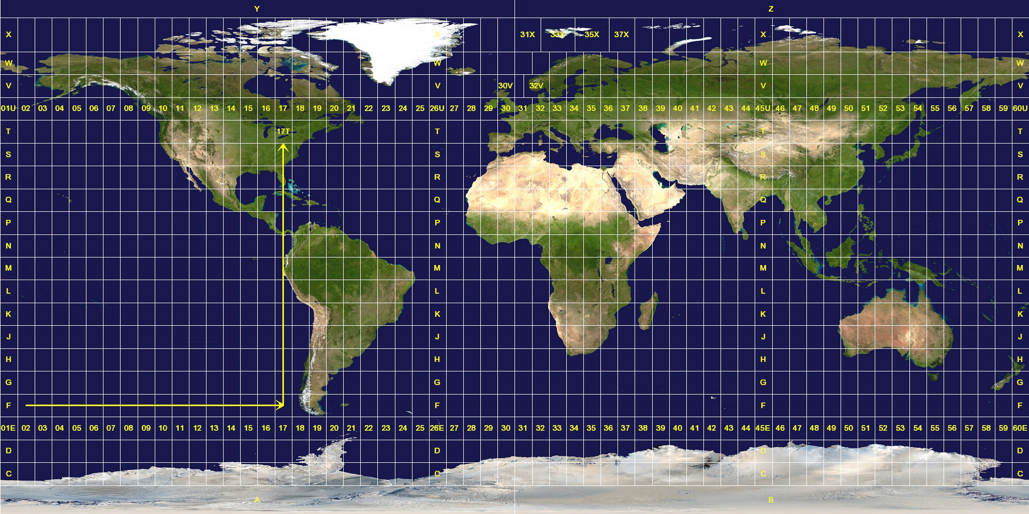
zone |
UTM (Universal Transverse Mercator) zone, see e.g.
https://upload.wikimedia.org/wikipedia/commons/e/ed/Utm-zones.jpg.
DEFAULT: UTM zone at mean of |
map |
for pmap: map object as returned by |
Value
sf::st_crs objects for one of:
- UTM projection with given zone
- Open street map (and google) mercator projection
- Latitude Longitude projection
Author(s)
Berry Boessenkool, berry-b@gmx.de, Aug 2016
See Also
Examples
posm()
str(posm())
pll()
putm(5:14) # Germany
putm(zone=33) # Berlin

map <- list(tiles=list(dummy=list(projection=pll())),
            bbox=list(p1=par("usr")[c(1,4)], p2=par("usr")[2:3]) )
pmap(map)
Project lat-lon points
Description
Project long lat points to e.g. UTM projection.
Basics copied from OpenStreetMap::projectMercator
Usage
projectPoints(
  lat,
  long,
  data,
  from = pll(),
  to = putm(long = long),
  dfout = TRUE,
  drop = FALSE,
  quiet = FALSE
)
Arguments
lat, long |
Latitude (North/South) and longitude (East/West) coordinates in decimal degrees |
data |
Optional: data.frame with the columns |
from |
Original Projection CRS (do not change for latlong-coordinates).
DEFAULT: |
to |
target projection CRS (Coordinate Reference System) Object.
Other projections can be specified as |
dfout |
Convert output to data.frame to allow easier indexing? DEFAULT: TRUE |
drop |
Drop to lowest dimension? DEFAULT: FALSE (unlike |
quiet |
Suppress warning about NA coordinates and non-df warning in
|
Value
data.frame (or matrix, if dfout=FALSE) with points in new projection
Author(s)
Berry Boessenkool, berry-b@gmx.de, Jun 2016
See Also
scaleBar, OpenStreetMap::projectMercator,
https://gis.stackexchange.com/a/74723, https://spatialreference.org on proj4strings
Examples
library("OpenStreetMap")
lat <- runif(100, 6, 12)
lon <- runif(100, 48, 58)
plot(lat,lon, main="flat earth unprojected")
plot(projectMercator(lat,lon), main="Mercator")
plot(projectPoints(lat,lon), main="UTM32")
stopifnot(all( projectPoints(lat,lon, to=posm()) == projectMercator(lat,lon) ))

projectPoints(c(52.4,NA),      c(13.6,12.9))
projectPoints(c(52.4,NA),      c(13.6,12.9), quiet=TRUE)
projectPoints(c(52.4,52.3,NA), c(13.6,12.9,13.1))
projectPoints(c(52.4,52.3,NA), c(13.6,NA  ,13.1))
projectPoints(c(52.4,52.3,NA), c(NA  ,12.9,13.1))

# Reference system ETRS89 with GRS80-Ellipsoid (common in Germany)
set.seed(42)
d <- data.frame(N=runif(50,5734000,6115000), E=runif(50, 33189000,33458000))
d$VALUES <- berryFunctions::rescale(d$N, 20,40) + rnorm(50, sd=5)
head(d)
c1 <- projectPoints(lat=d$N, long=d$E-33e6, to=pll(),
          from=sf::st_crs("+proj=utm +zone=33 +ellps=GRS80 +units=m +no_defs") )
c2 <- projectPoints(y, x, data=c1, to=posm() )
head(c1)
head(c2)

## Not run:  # not checked on CRAN because of file opening
map <- pointsMap(y,x, c1, plot=FALSE)
if(!is.character(map)){ # failed maps return a character string
pdf("ETRS89.pdf")
par(mar=c(0,0,0,0))
plot(map)
rect(par("usr")[1], par("usr")[3], par("usr")[2], par("usr")[4],
     col=berryFunctions::addAlpha("white", 0.7))
scaleBar(map, y=0.2, abslen=100)
points(c2)
berryFunctions::colPoints(c2$x, c2$y, d$VALUE )
dev.off()
berryFunctions::openFile("ETRS89.pdf")
#unlink("ETRS89.pdf")
}

## End(Not run)
Distanced random points
Description
Arranges points in square randomly, but with certain minimal distance to each other
Usage
randomPoints(xmin, xmax, ymin, ymax, number, mindist, plot = TRUE, ...)
Arguments
xmin |
Minimum x coordinate |
xmax |
Upper limit x values |
ymin |
Ditto for y |
ymax |
And yet again: Ditto. |
number |
How many points should be randomly + uniformly distributed |
mindist |
Minimum DIstance each point should have to others |
plot |
Plot the result? DEFAULT: TRUE |
... |
Further arguments passed to plot |
Value
data.frame with x and y coordinates.
Author(s)
Berry Boessenkool, berry-b@gmx.de, 2011/2012
See Also
berryFunctions::distance,
the package RandomFields ( https://cran.r-project.org/package=RandomFields)
Examples
P <- randomPoints(xmin=200,xmax=700, ymin=300,ymax=680, number=60,mindist=10, asp=1)
rect(xleft=200, ybottom=300, xright=700, ytop=680, col=NA, border=1)

format( round(P,4), trim=FALSE)

for(i in 1:10)
{
rp <- randomPoints(xmin=0,xmax=20, ymin=0,ymax=20, number=20, mindist=3, plot=FALSE)
plot(rp, las=1, asp=1, pch=16)
abline(h=0:30*2, v=0:30*2, col=8); box()
for(i in 1:nrow(rp))
    berryFunctions::circle(rp$x[i],rp$y[i], r=3, col=rgb(1,0,0,alpha=0.2), border=NA)
}
scalebar for OSM plots
Description
Add a scalebar to default or (UTM)-projected OpenStreetMap plots
Usage
scaleBar(
  map,
  x = 0.1,
  y = 0.9,
  length = 0.4,
  abslen = NA,
  unit = c("km", "m", "mi", "ft", "yd"),
  label = unit,
  type = c("bar", "line"),
  ndiv = NA,
  field = "rect",
  fill = NA,
  adj = c(0.5, 1.5),
  cex = par("cex"),
  col = c("black", "white"),
  targs = NULL,
  lwd = 7,
  lend = 1,
  bg = "transparent",
  mar = c(2, 0.7, 0.2, 3),
  ...
)
Arguments
map |
Map object with map$tiles[[1]]$projection to get the projection from. |
x, y |
Relative position of left end of scalebar. DEFAULT: 0.1, 0.9 |
length |
Approximate relative length of bar. DEFAULT: 0.4 |
abslen |
Absolute length in |
unit |
Unit for computation and label. Possible: kilometer, meter, miles, feet, yards. DEFAULT: "km" |
label |
Unit label in plot. DEFAULT: |
type |
Scalebar type: simple |
ndiv |
Number of divisions if |
field, fill, adj, cex |
Arguments passed to |
col |
Vector of (possibly alternating) colors passed to
|
targs |
List of further arguments passed to |
lwd, lend |
Line width and end style passed to |
bg |
Background color, e.g. |
mar |
Background margins approximately in letter width/height. DEFAULT: c(2,0.7,0.2,3) |
... |
Further arguments passed to |
Details
scaleBar gets the right distance in the default mercator projected maps. There, the axes are not in meters, but rather ca 0.7m units (for NW Germany area maps with 20km across). Accordingly, other packages plot wrong bars, see the last example section.
Value
invisible: coordinates of scalebar and label
Author(s)
Berry Boessenkool, berry-b@gmx.de, Jun 2016
See Also
Examples
plot(0:10, 40:50, type="n", asp=1) # Western Europe in lat-long
map <- list(tiles=list(dummy=list(projection=pll())),
            bbox=list(p1=par("usr")[c(1,4)], p2=par("usr")[2:3]) )
scaleBar(map)

if(interactive()){
d <- data.frame(long=c(12.95, 12.98, 13.22, 13.11), lat=c(52.40,52.52, 52.36, 52.45))
map <- pointsMap(lat,long,d, scale=FALSE, zoom=9)
if(!is.character(map)){ # failed maps return a character string
coord <- scaleBar(map)  ; coord
scaleBar(map, bg=berryFunctions::addAlpha("white", 0.7))
scaleBar(map, 0.3, 0.05, unit="m", length=0.45, type="line")
scaleBar(map, 0.3, 0.5, unit="km", abslen=5, col=4:5, lwd=3)
scaleBar(map, 0.3, 0.8, unit="mi", col="red", targ=list(col="blue", font=2), type="line")

# I don't like subdivisions, but if you wanted them, you could use:
sb <- scaleBar(map, 0.12, 0.28, abslen=10, adj=c(0.5, -1.5)  )
scaleBar(map, 0.12, 0.28, abslen=4, adj=c(0.5, -1.5),
         targs=list(col="transparent"), label="" )

# more lines for exact measurements in scalebar:
segments(x0=seq(sb["x1"], sb["x2"], len=21), y0=sb["y1"], y1=sb["y2"], col=8)
rect(xleft=sb["x1"], xright=sb["x2"], ybottom=sb["y1"], ytop=sb["y2"])
}
}

## Not run:  # don't download too many maps in R CMD check
d <- read.table(header=TRUE, sep=",", text="
lat, long
52.514687,  13.350012   # Berlin
51.503162,  -0.131082   # London
35.685024, 139.753365") # Tokio
map <- pointsMap(lat, long, d, zoom=2, abslen=5000, y=0.7)
if(!is.character(map)){ # failed maps return a character string
scaleBar(map, y=0.5, abslen=5000)   # in mercator projections, scale bars are not
scaleBar(map, y=0.3, abslen=5000)   # transferable to other latitudes

map_utm <- pointsMap(lat, long, d[1:2,], proj=putm(long=d$long[1:2]),
                     zoom=4, y=0.7, abslen=500)
scaleBar(map_utm, y=0.5, abslen=500) # transferable in UTM projection
scaleBar(map_utm, y=0.3, abslen=500)
}

## End(Not run)

## Not run:  ## Too much downloading time, too error-prone
# Tests around the world
par(mfrow=c(1,2), mar=rep(1,4))
long <- runif(2, -180, 180) ;  lat <- runif(2, -90, 90)
long <- 0:50 ;  lat <- 0:50
map <- pointsMap(lat, long)
if(!is.character(map)) # failed maps return a character string
map2 <- pointsMap(lat, long, map=map, proj=putm(long=long))

## End(Not run)

## Not run:  ## excluded from tests to avoid package dependencies
# berryFunctions::require2("SDMTools")
berryFunctions::require2("raster")
berryFunctions::require2("mapmisc")
par(mar=c(0,0,0,0))
map <- OSMscale::pointsMap(long=c(12.95, 13.22), lat=c(52.52, 52.36))
if(!is.character(map)){ # failed maps return a character string
# SDMTools::Scalebar(x=1443391,y=6889679,distance=10000)
raster::scalebar(d=10000, xy=c(1443391,6884254))
OSMscale::scaleBar(map, x=0.35, y=0.45, abslen=5)
library(mapmisc) # otherwise rbind for SpatialPoints is not found
mapmisc::scaleBar(pmap(map)@projargs, seg.len=10, pos="center", bg="transparent")
}

## End(Not run)
Area of a triangle
Description
calculate Area of a planar triangle
Usage
triangleArea(x, y, digits = 3)
Arguments
x |
Vector with 3 values (x coordinates of triangle corners) |
y |
Ditto for y. |
digits |
Number of digits the result is rounded to. DEFAULT: 3) |
Value
Numeric
Author(s)
Berry Boessenkool, berry-b@gmx.de, 2011
See Also
berryFunctions::distance
Examples
a <- c(1,5.387965,9); b <- c(1,1,5)
plot(a[c(1:3,1)], b[c(1:3,1)], type="l", asp=1)#; grid()

triangleArea(a,b)
#triangleArea(a,b[1:2])