| Title: | Robust and User-Friendly Analysis of Growth and Fluorescence Curves |
| Version: | 1.1.2 |
| Description: | High-throughput analysis of growth curves and fluorescence data using three methods: linear regression, growth model fitting, and smooth spline fit. Analysis of dose-response relationships via smoothing splines or dose-response models. Complete data analysis workflows can be executed in a single step via user-friendly wrapper functions. The results of these workflows are summarized in detailed reports as well as intuitively navigable 'R' data containers. A 'shiny' application provides access to all features without requiring any programming knowledge. The package is described in further detail in Wirth et al. (2023) <doi:10.1038/s41596-023-00850-7>. |
| License: | GPL (≥ 3) |
| URL: | https://github.com/NicWir/QurvE, https://nicwir.github.io/QurvE/ |
| BugReports: | https://github.com/NicWir/QurvE/issues |
| Depends: | dplyr, methods, R (≥ 4.0), stringr, tidyr |
| Imports: | doParallel, drc, DT, foreach, ggh4x, ggnewscale, ggplot2, ggpubr, kableExtra, knitr, labeling, magrittr, minpack.lm, plyr, purrr, RColorBrewer, readxl, rmarkdown, scales, shiny, stats, utils |
| Suggests: | bookdown, Cairo, htmltools, plotrix, prettydoc, rlang, shinyBS, shinycssloaders, shinyFiles, shinyjs, shinythemes, testthat (≥ 3.0.0), tibble, tinytex |
| VignetteBuilder: | knitr |
| Encoding: | UTF-8 |
| RoxygenNote: | 7.3.3 |
| Collate: | 'QurvE-package.R' 'control_functions.R' 'data_parsers.R' 'dose-response-analysis.R' 'fluorescence_plots.R' 'fluorescence_summaries.R' 'fluorescence_workflows.R' 'group_tables.R' 'utils.R' 'growth_plots.R' 'growth_summaries.R' 'growth_workflows.R' 'linear_fits.R' 'nonparametric_fits.R' 'parametric_fits.R' 'report_functions.R' 'shiny_app_functions.R' |
| NeedsCompilation: | no |
| Packaged: | 2025-09-19 13:20:23 UTC; ncw |
| Author: | Nicolas T. Wirth  [aut, cre, cph],
Jonathan Funk [aut] (contribution: Co-developer of shiny app.),
Matthias Kahm [ctb] (contribution: Author of 'grofit' package, whose
general data structure was adopted for QurvE.),
Maik Kschischo [ctb] (contribution: Author of 'grofit' package, whose
general data structure was adopted for QurvE.),
Thomas Petzoldt
[ctb] (contribution: Creator of the package 'growthrates', whose
function for calculating linear regressions served as a template in
QurvE.),
Andrew Stein [ctb] (contribution: Creator of 'xgxr' package from which
QurvE adopted code to plot axis ticks on log10 scale.),
Michael W. Kearney [ctb] (contribution: Creator of 'tfse' package from
which QurvE adopted the match_arg function.),
Santiago I. Hurtado [ctb] (contribution: Creator of 'RobustLinearReg'
package from which QurvE adopted the Theil Sehn Regression method.),
Mark Heckmann [ctb] (contribution: Creator of the 'zipFastener'
function; source:
https://ryouready.wordpress.com/2009/03/27/r-zip-fastener-for-two-data-frames-combining-rows-or-columns-of-two-dataframes-in-an-alternating-manner/),
Nicholas Hamilton [ctb] (contribution: Creator of the 'colFmt'
function.),
Evan Friedland [ctb] (contribution: Creator of the 'inflect' function.),
Heather Turner [ctb] (contribution: Creator of the 'base_breaks'
function.),
Georgi N. Boshnakov [ctb] (contribution: Creator of 'gbRd' package from
which functions are used to display function help pages within the
shiny app.)
[aut, cre, cph],
Jonathan Funk [aut] (contribution: Co-developer of shiny app.),
Matthias Kahm [ctb] (contribution: Author of 'grofit' package, whose
general data structure was adopted for QurvE.),
Maik Kschischo [ctb] (contribution: Author of 'grofit' package, whose
general data structure was adopted for QurvE.),
Thomas Petzoldt
[ctb] (contribution: Creator of the package 'growthrates', whose
function for calculating linear regressions served as a template in
QurvE.),
Andrew Stein [ctb] (contribution: Creator of 'xgxr' package from which
QurvE adopted code to plot axis ticks on log10 scale.),
Michael W. Kearney [ctb] (contribution: Creator of 'tfse' package from
which QurvE adopted the match_arg function.),
Santiago I. Hurtado [ctb] (contribution: Creator of 'RobustLinearReg'
package from which QurvE adopted the Theil Sehn Regression method.),
Mark Heckmann [ctb] (contribution: Creator of the 'zipFastener'
function; source:
https://ryouready.wordpress.com/2009/03/27/r-zip-fastener-for-two-data-frames-combining-rows-or-columns-of-two-dataframes-in-an-alternating-manner/),
Nicholas Hamilton [ctb] (contribution: Creator of the 'colFmt'
function.),
Evan Friedland [ctb] (contribution: Creator of the 'inflect' function.),
Heather Turner [ctb] (contribution: Creator of the 'base_breaks'
function.),
Georgi N. Boshnakov [ctb] (contribution: Creator of 'gbRd' package from
which functions are used to display function help pages within the
shiny app.) |
| Maintainer: | Nicolas T. Wirth <mail.nicowirth@gmail.com> |
| Repository: | CRAN |
| Date/Publication: | 2025-09-19 13:40:13 UTC |
QurvE: Robust and User-Friendly Analysis of Growth and Fluorescence Curves
Description
High-throughput analysis of growth curves and fluorescence data using three methods: linear regression, growth model fitting, and smooth spline fit. Analysis of dose-response relationships via smoothing splines or dose-response models. Complete data analysis workflows can be executed in a single step via user-friendly wrapper functions. The results of these workflows are summarized in detailed reports as well as intuitively navigable 'R' data containers. A 'shiny' application provides access to all features without requiring any programming knowledge. The package is described in further detail in Wirth et al. (2023) doi:10.1038/s41596-023-00850-7.
Author(s)
Maintainer: Nicolas T. Wirth mail.nicowirth@gmail.com (ORCID) [copyright holder]
Authors:
Jonathan Funk funk.jonathan21@gmail.com (Co-developer of shiny app.)
Other contributors:
Matthias Kahm (Author of 'grofit' package, whose general data structure was adopted for QurvE.) [contributor]
Maik Kschischo (Author of 'grofit' package, whose general data structure was adopted for QurvE.) [contributor]
Thomas Petzoldt thomas.petzoldt@tu-dresden.de (ORCID) (Creator of the package 'growthrates', whose function for calculating linear regressions served as a template in QurvE.) [contributor]
Andrew Stein andy.stein@gmail.com (Creator of 'xgxr' package from which QurvE adopted code to plot axis ticks on log10 scale.) [contributor]
Michael W. Kearney kearneymw@missouri.edu (Creator of 'tfse' package from which QurvE adopted the match_arg function.) [contributor]
Santiago I. Hurtado santih@carina.fcaglp.unlp.edu.ar (Creator of 'RobustLinearReg' package from which QurvE adopted the Theil Sehn Regression method.) [contributor]
Mark Heckmann (Creator of the 'zipFastener' function; source: https://ryouready.wordpress.com/2009/03/27/r-zip-fastener-for-two-data-frames-combining-rows-or-columns-of-two-dataframes-in-an-alternating-manner/) [contributor]
Nicholas Hamilton (Creator of the 'colFmt' function.) [contributor]
Evan Friedland (Creator of the 'inflect' function.) [contributor]
Heather Turner (Creator of the 'base_breaks' function.) [contributor]
Georgi N. Boshnakov georgi.boshnakov@manchester.ac.uk (Creator of 'gbRd' package from which functions are used to display function help pages within the shiny app.) [contributor]
See Also
Useful links:
Report bugs at https://github.com/NicWir/QurvE/issues
A palette with 40 colors
Description
This palette is used in the package for plotting.
Usage
big_palette
Format
An object of class character of length 50.
Internal function used to fit a biosensor response model with nlsLM
Description
Calculates the values of biosensor response model for given time points and response parameters.
Usage
biosensor.eq(x, y.min, y.max, K, n)
Arguments
x |
A vector of concentration values |
y.min |
The minimum fluorescence value |
y.max |
The maximum fluorescence value |
K |
Sensitivity parameter |
n |
Cooperativity parameter |
Value
A vector of fluorescence values
References
Meyer, A.J., Segall-Shapiro, T.H., Glassey, E. et al. Escherichia coli “Marionette” strains with 12 highly optimized small-molecule sensors. Nat Chem Biol 15, 196–204 (2019). DOI: 10.1038/s41589-018-0168-3
Examples
n <- seq(1:10)
conc <- rev(10*(1/2)^n)
fit <- biosensor.eq(conc, 300, 82000, 0.85, 2)
Custom tooltip function
Description
This function creates a custom tooltip for a given element in a Shiny application. The implementation is based on the shinyBS package.
Usage
buildTooltipOrPopoverOptionsList(title, placement, trigger, options, content)
Arguments
title |
The text for the tooltip's title. |
placement |
Placement of the tooltip. One of 'top', 'bottom', 'left', or 'right'. |
trigger |
The events that trigger the tooltip. One or more of 'click', 'hover', 'focus', or 'manual'. |
options |
A list of additional options for the tooltip. |
content |
Optional HTML content for the tooltip. |
Value
A list of tooltip options to be used in the Shiny application.
See Also
https://CRAN.R-project.org/package=shinyBS
Examples
## Not run:
tooltip_options <- custom_tooltip(
  title = "Sample tooltip",
  placement = "top",
  trigger = "hover",
  options = list(delay = 100),
  content = "This is a custom tooltip."
)

# In a Shiny app
# shiny::tags$span("Hover me!", `data-toggle` = "tooltip",
                   `data-placement` = "top", `data-trigger` = "hover",
                   `title` = "Hello, tooltip!")

## End(Not run)
Export an R object as .RData file
Description
Export an R object as .RData file
Usage
export_RData(object, out.dir = tempdir(), out.nm = class(object))
Arguments
object |
An R object. |
out.dir |
The path to the output directory. Default: the working directory |
out.nm |
The output filename (with or without '.RData' ending). Default: the class of |
Value
NULL
Examples
if(interactive()){
df <- data.frame('A' = seq(1:10), 'B' = rev(seq(1:10)))

export_RData(df)
}
Export a tabular object as tab-separated .txt file
Description
Export a tabular object as tab-separated .txt file
Usage
export_Table(table, out.dir = tempdir(), out.nm = deparse(substitute(table)))
Arguments
table |
A tabular R object (dataframe, matrix, array) |
out.dir |
The path to the output directory. Default: the working directory |
out.nm |
The output filename (with or without '.txt' ending). Default: the name of |
Value
NULL
Examples
if(interactive()){
df <- data.frame('A' = seq(1:10), 'B' = rev(seq(1:10)))

export_Table(df)
}
Create a fl.control object.
Description
A fl.control object is required to perform various computations on fluorescence data stored within grodata objects (created with read_data or parse_data). A fl.control object is created automatically as part of fl.workflow.
Usage
fl.control(
  fit.opt = c("l", "s"),
  x_type = c("growth", "time"),
  norm_fl = TRUE,
  t0 = 0,
  tmax = NA,
  min.growth = NA,
  max.growth = NA,
  log.x.lin = FALSE,
  log.x.spline = FALSE,
  log.y.lin = FALSE,
  log.y.spline = FALSE,
  lin.h = NULL,
  lin.R2 = 0.97,
  lin.RSD = 0.05,
  lin.dY = 0.05,
  dr.parameter = "max_slope.spline",
  dr.method = c("model", "spline"),
  dr.have.atleast = 5,
  smooth.dr = NULL,
  log.x.dr = FALSE,
  log.y.dr = FALSE,
  nboot.dr = 0,
  biphasic = FALSE,
  interactive = FALSE,
  nboot.fl = 0,
  smooth.fl = 0.75,
  growth.thresh = 1.5,
  suppress.messages = FALSE,
  neg.nan.act = FALSE,
  clean.bootstrap = TRUE
)
Arguments
fit.opt |
(Character or vector of strings) Indicates whether the program should perform a linear regression ( |
x_type |
(Character) Which data type shall be used as independent variable? Options are |
norm_fl |
(Logical) use normalized (to growth) fluorescence data in fits. Has an effect only when |
t0 |
(Numeric) Minimum time value considered for linear and spline fits (if |
tmax |
(Numeric) Maximum time value considered for linear and spline fits (if |
min.growth |
(Numeric) Indicate whether only values above a certain threshold should be considered for linear regressions or spline fits (if |
max.growth |
(Numeric) Indicate whether only growth values below a certain threshold should be considered for linear regressions or spline fits (if |
log.x.lin |
(Logical) Indicates whether ln(x+1) should be applied to the independent variable for linear fits. Default: |
log.x.spline |
(Logical) Indicates whether ln(x+1) should be applied to the independent variable for spline fits. Default: |
log.y.lin |
(Logical) Indicates whether ln(y/y0) should be applied to the fluorescence data for linear fits. Default: |
log.y.spline |
(Logical) Indicates whether ln(y/y0) should be applied to the fluorescence data for spline fits. Default: |
lin.h |
(Numeric) Manually define the size of the sliding window used in |
lin.R2 |
(Numeric) R2 threshold for |
lin.RSD |
(Numeric) Relative standard deviation (RSD) threshold for the calculated slope in |
lin.dY |
(Numeric) Threshold for the minimum fraction of growth increase a linear regression window should cover. Default: 0.05 (5%). |
dr.parameter |
(Character or numeric) The response parameter in the output table to be used for creating a dose response curve. See |
dr.method |
(Character) Perform either a smooth spline fit on response parameter vs. concentration data ( |
dr.have.atleast |
(Numeric) Minimum number of different values for the response parameter one should have for estimating a dose response curve. Note: All fit procedures require at least six unique values. Default: |
smooth.dr |
(Numeric) Smoothing parameter used in the spline fit by smooth.spline during dose response curve estimation. Usually (not necessesary) in (0; 1]. See |
log.x.dr |
(Logical) Indicates whether |
log.y.dr |
(Logical) Indicates whether |
nboot.dr |
(Numeric) Defines the number of bootstrap samples for EC50 estimation. Use |
biphasic |
(Logical) Shall |
interactive |
(Logical) Controls whether the fit for each sample and method is controlled manually by the user. If |
nboot.fl |
(Numeric) Number of bootstrap samples used for nonparametric curve fitting with |
smooth.fl |
(Numeric) Parameter describing the smoothness of the spline fit; usually (not necessary) within (0;1]. |
growth.thresh |
(Numeric) Define a threshold for growth. Only if any growth value in a sample is greater than |
suppress.messages |
(Logical) Indicates whether messages (information about current fluorescence curve, EC50 values etc.) should be displayed ( |
neg.nan.act |
(Logical) Indicates whether the program should stop when negative fluorescence values or NA values appear ( |
clean.bootstrap |
(Logical) Determines if negative values which occur during bootstrap should be removed ( |
Value
Generates a list with all arguments described above as entries.
References
Meyer, A.J., Segall-Shapiro, T.H., Glassey, E. et al. Escherichia coli “Marionette” strains with 12 highly optimized small-molecule sensors. Nat Chem Biol 15, 196–204 (2019). DOI: 10.1038/s41589-018-0168-3
Examples
# default option
control_default <- fl.control()
# user defined
control_manual <- fl.control(fit.opt = c('s'),
                             smooth.fl = 0.6,
                             x_type = 'time',
                             t0 = 2)
Fit a biosensor model (Meyer et al., 2019) to response vs. concentration data
Description
Fit a biosensor model (Meyer et al., 2019) to response vs. concentration data
Usage
fl.drFit(
  flTable,
  control = fl.control(dr.method = "model", dr.parameter = "max_slope.spline")
)
Arguments
flTable |
A dataframe containing the data for the dose-response model estimation. Such table of class |
control |
A |
dr.method |
(Character) Perform either a smooth spline fit on response parameter vs. concentration data ( |
dr.parameter |
(Character or numeric) The response parameter in the output table to be used for creating a dose response curve. See |
Details
Common response parameters used in dose-response analysis:
Linear fit:
- max_slope.linfit: Fluorescence increase rate
- lambda.linfit: Lag time
- dY.linfit: Maximum Fluorescence - Minimum Fluorescence
- A.linfit: Maximum fluorescence
Spline fit:
- max_slope.spline: Fluorescence increase rate
- lambda.spline: Lag time
- dY.spline: Maximum Fluorescence - Minimum Fluorescence
- A.spline: Maximum fluorescence
- integral.spline: Integral
Parametric fit:
- max_slope.model: Fluorescence increase rate
- lambda.model: Lag time
- dY.model: Maximum Fluorescence - Minimum Fluorescence
- A.model: Maximum fluorescence
- integral.model: Integral'
Value
An object of class drFit.
raw.data |
Data that passed to the function as |
drTable |
Dataframe containing condition identifiers, fit options, and results of the dose-response analysis. |
drFittedModels |
List of all |
control |
Object of class |
References
Meyer, A.J., Segall-Shapiro, T.H., Glassey, E. et al. Escherichia coli “Marionette” strains with 12 highly optimized small-molecule sensors. Nat Chem Biol 15, 196–204 (2019). DOI: 10.1038/s41589-018-0168-3
Examples
# Load example dataset
input <- read_data(data.fl = system.file('lac_promoters_fluorescence.txt', package = 'QurvE'),
                   csvsep.fl = "\t")

# Run fluorescence curve analysis workflow
fitres <- flFit(fl_data = input$fluorescence,
                time = input$time,
                parallelize = FALSE,
                control = fl.control(x_type = 'time', norm_fl = FALSE,
                                     suppress.messages = TRUE))

# Perform dose-response analysis
drFit <- fl.drFit(flTable = fitres$flTable,
                  control = fl.control(dr.method = 'model',
                                       dr.parameter = 'max_slope.linfit'))

# Inspect results
summary(drFit)
plot(drFit)
Perform a biosensor model fit on response vs. concentration data of a single sample.
Description
fl.drFitModel fits the biosensor model proposed by Meyer et al. (2019) to the provided response (e.g., max_slope.spline vs. concentration data to determine the leakiness, sensitivity, induction fold-change, and cooperativity.
Usage
fl.drFitModel(conc, test, drID = "undefined", control = fl.control())
Arguments
conc |
Vector of concentration values. |
test |
Vector of response parameter values of the same length as |
drID |
(Character) The name of the analyzed condition |
control |
A |
Value
A drFitFLModel object.
raw.conc |
Raw data provided to the function as |
raw.test |
Raw data for the response parameter provided to the function as |
drID |
(Character) Identifies the tested condition |
fit.conc |
Fitted concentration values. |
fit.test |
Fitted response values. |
model |
|
parameters |
List of parameters estimated from dose response curve fit. |
-
yEC50: Response value related to EC50. -
y.min: Minimum fluorescence ('leakiness', if lowest concentration is 0). -
y.max: Maximum fluorescence. -
fc: Fold change (y.maxdivided byy.min). -
K: Concentration at half-maximal response ('sensitivity'). -
n: Cooperativity. -
yEC50.orig: Response value for EC50 in original scale, if a transformation was applied. -
K.orig: K in original scale, if a transformation was applied. -
test.nm: Test identifier extracted fromtest.
fitFlag |
(Logical) Indicates whether a spline could fitted successfully to data. |
reliable |
(Logical) Indicates whether the performed fit is reliable (to be set manually). |
control |
Object of class |
Use plot.drFitModel to visualize the model fit.
References
Meyer, A.J., Segall-Shapiro, T.H., Glassey, E. et al. Escherichia coli “Marionette” strains with 12 highly optimized small-molecule sensors. Nat Chem Biol 15, 196–204 (2019). DOI: 10.1038/s41589-018-0168-3
Examples
# Create concentration values via a serial dilution
conc <- c(0, rev(unlist(lapply(1:18, function(x) 10*(2/3)^x))),10)

# Simulate response values via biosensor equation
response <- biosensor.eq(conc, y.min = 110, y.max = 6000, K = 0.5, n = 2) +
            0.01*6000*rnorm(10)

# Perform fit
TestRun <- fl.drFitModel(conc, response, drID = 'test', control = fl.control())

print(summary(TestRun))
plot(TestRun)
Create a PDF and HTML report with results from a fluorescence analysis workflow
Description
fl.report requires a flFitRes object and creates a report in PDF and HTML format that summarizes all results obtained.
Usage
fl.report(
  flFitRes,
  out.dir = tempdir(),
  out.nm = NULL,
  ec50 = FALSE,
  format = c("pdf", "html"),
  export = FALSE,
  parallelize = TRUE,
  ...
)
Arguments
flFitRes |
A |
out.dir |
(Character) The path or name of the folder in which the report files are created. If |
out.nm |
Character or |
ec50 |
(Logical) Display results of dose-response analysis ( |
format |
(Character) Define the file format for the report, PDF ( |
export |
(Logical) Shall all plots generated in the report be exported as individual PDF and PNG files |
parallelize |
(Logical) Create plots using all but one available processor cores ( |
... |
Further arguments passed to create a report. Currently supported:
|
Details
The template .Rmd file used within this function can be found within the QurvE package installation directory.
Value
NULL
Examples
# load example dataset
## Not run:
input <- read_data(data.growth = system.file("lac_promoters_growth.txt", package = "QurvE"),
                   data.fl = system.file("lac_promoters_fluorescence.txt", package = "QurvE"),
                   csvsep = "\t",
                   csvsep.fl = "\t")

# Run workflow
res <- fl.workflow(grodata = input, ec50 = FALSE, fit.opt = 's',
                   x_type = 'time', norm_fl = TRUE,
                   dr.parameter = 'max_slope.spline',
                   suppress.messages = TRUE,
                   parallelize = FALSE)

fl.report(res, out.dir = tempdir(), parallelize = FALSE)

## End(Not run)
Run a complete fluorescence curve analysis and dose-reponse analysis workflow.
Description
fl.workflow runs fl.control to create a fl.control object and then performs all computational fitting operations based on the user input. Finally, if desired, a final report is created in PDF or HTML format that summarizes all results obtained.
Usage
fl.workflow(
  grodata = NULL,
  time = NULL,
  growth = NULL,
  fl_data = NULL,
  ec50 = TRUE,
  mean.grp = NA,
  mean.conc = NA,
  fit.opt = c("l", "s"),
  x_type = c("growth", "time"),
  norm_fl = TRUE,
  t0 = 0,
  tmax = NA,
  min.growth = 0,
  max.growth = NA,
  log.x.lin = FALSE,
  log.x.spline = FALSE,
  log.y.lin = FALSE,
  log.y.spline = FALSE,
  lin.h = NULL,
  lin.R2 = 0.97,
  lin.RSD = 0.07,
  lin.dY = 0.05,
  biphasic = FALSE,
  interactive = FALSE,
  dr.parameter = "max_slope.spline",
  dr.method = c("model", "spline"),
  dr.have.atleast = 5,
  smooth.dr = NULL,
  log.x.dr = FALSE,
  log.y.dr = FALSE,
  nboot.dr = 0,
  nboot.fl = 0,
  smooth.fl = 0.75,
  growth.thresh = 1.5,
  suppress.messages = FALSE,
  neg.nan.act = FALSE,
  clean.bootstrap = TRUE,
  report = NULL,
  out.dir = NULL,
  out.nm = NULL,
  export.fig = FALSE,
  export.res = FALSE,
  parallelize = TRUE,
  ...
)
Arguments
grodata |
A |
time |
(optional) A matrix containing time values for each sample (if a |
growth |
(optional) A dataframe containing growth data (if a |
fl_data |
(optional) A dataframe containing fluorescence data (if a |
ec50 |
(Logical) Perform dose-response analysis ( |
mean.grp |
( |
mean.conc |
(A numeric vector, or a list of numeric vectors) Define concentrations to combine into common plots in the final report (if |
fit.opt |
(Character or character vector) Indicates whether the program should perform a linear regression ( |
x_type |
(Character) Which data type shall be used as independent variable? Options are |
norm_fl |
(Logical) use normalized (to growth) fluorescence data in fits. Has an effect only when |
t0 |
(Numeric) Minimum time value considered for linear and spline fits (if |
tmax |
(Numeric) Maximum time value considered for linear and spline fits (if |
min.growth |
(Numeric) Indicate whether only values above a certain threshold should be considered for linear regressions or spline fits (if |
max.growth |
(Numeric) Indicate whether only growth values below a certain threshold should be considered for linear regressions or spline fits (if |
log.x.lin |
(Logical) Indicates whether ln(x+1) should be applied to the independent variable for linear fits. Default: |
log.x.spline |
(Logical) Indicates whether ln(x+1) should be applied to the independent variable for spline fits. Default: |
log.y.lin |
(Logical) Indicates whether ln(y/y0) should be applied to the fluorescence data for linear fits. Default: |
log.y.spline |
(Logical) Indicates whether ln(y/y0) should be applied to the fluorescence data for spline fits. Default: |
lin.h |
(Numeric) Manually define the size of the sliding window used in |
lin.R2 |
(Numeric) R2 threshold for |
lin.RSD |
(Numeric) Relative standard deviation (RSD) threshold for the calculated slope in |
lin.dY |
(Numeric) Threshold for the minimum fraction of growth increase a linear regression window should cover. Default: 0.05 (5%). |
biphasic |
(Logical) Shall |
interactive |
(Logical) Controls whether the fit for each sample and method is controlled manually by the user. If |
dr.parameter |
(Character or numeric) The response parameter in the output table to be used for creating a dose response curve. See |
dr.method |
(Character) Perform either a smooth spline fit on response parameter vs. concentration data ( |
dr.have.atleast |
(Numeric) Minimum number of different values for the response parameter one should have for estimating a dose response curve. Note: All fit procedures require at least six unique values. Default: |
smooth.dr |
(Numeric) Smoothing parameter used in the spline fit by smooth.spline during dose response curve estimation. Usually (not necessesary) in (0; 1]. See |
log.x.dr |
(Logical) Indicates whether |
log.y.dr |
(Logical) Indicates whether |
nboot.dr |
(Numeric) Defines the number of bootstrap samples for EC50 estimation. Use |
nboot.fl |
(Numeric) Number of bootstrap samples used for nonparametric curve fitting with |
smooth.fl |
(Numeric) Parameter describing the smoothness of the spline fit; usually (not necessary) within (0;1]. |
growth.thresh |
(Numeric) Define a threshold for growth. Only if any growth value in a sample is greater than |
suppress.messages |
(Logical) Indicates whether messages (information about current fluorescence curve, EC50 values etc.) should be displayed ( |
neg.nan.act |
(Logical) Indicates whether the program should stop when negative fluorescence values or NA values appear ( |
clean.bootstrap |
(Logical) Determines if negative values which occur during bootstrap should be removed ( |
report |
(Character or NULL) Create a PDF ( |
out.dir |
Character or |
out.nm |
Character or |
export.fig |
(Logical) Export all figures created in the report as separate PNG and PDF files ( |
export.res |
(Logical) Create tab-separated TXT files containing calculated parameters and dose-response analysis results as well as an .RData file for the resulting |
parallelize |
Run linear fits and bootstrapping operations in parallel using all but one available processor cores |
... |
Further arguments passed to the shiny app. |
Value
A flFitRes object that contains all computation results, compatible with various plotting functions of the QurvE package and with fl.report.
time |
Raw time matrix passed to the function as |
data |
Raw data dataframe passed to the function as |
flFit |
|
drFit |
|
expdesign |
Experimental design table inherited from |
control |
Object of class |
Examples
# load example dataset
input <- read_data(data.growth = system.file("lac_promoters_growth.txt", package = "QurvE"),
                   data.fl = system.file("lac_promoters_fluorescence.txt", package = "QurvE"),
                   csvsep = "\t",
                   csvsep.fl = "\t")

# Run workflow
res <- fl.workflow(grodata = input, ec50 = FALSE, fit.opt = "s",
                   x_type = "time", norm_fl = TRUE,
                   dr.parameter = "max_slope.spline",
                   suppress.messages = TRUE,
                   parallelize = FALSE)

plot(res, data.type = "raw", legend.ncol = 3, basesize = 15)
flBootSpline: Function to generate a bootstrap
Description
fl.gcBootSpline resamples the fluorescence-'x' value pairs in a dataset with replacement and performs a spline fit for each bootstrap sample.
Usage
flBootSpline(
  time = NULL,
  growth = NULL,
  fl_data,
  ID = "undefined",
  control = fl.control()
)
Arguments
time |
Vector of the independent variable: time (if |
growth |
Vector of the independent variable: growth (if |
fl_data |
Vector of dependent variable: fluorescence. |
ID |
(Character) The name of the analyzed sample. |
control |
A |
Value
A gcBootSpline object containing a distribution of fluorescence parameters and
a flFitSpline object for each bootstrap sample. Use plot.gcBootSpline
to visualize all bootstrapping splines as well as the distribution of
physiological parameters.
raw.x |
Raw time values provided to the function as |
raw.fl |
Raw growth data provided to the function as |
ID |
(Character) Identifies the tested sample. |
boot.x |
Table of time values per column, resulting from each spline fit of the bootstrap. |
boot.fl |
Table of growth values per column, resulting from each spline fit of the bootstrap. |
boot.flSpline |
List of |
lambda |
Vector of estimated lambda (lag time) values from each bootstrap entry. |
max_slope |
Vector of estimated max_slope (maximum slope) values from each bootstrap entry. |
A |
Vector of estimated A (maximum fluorescence) values from each bootstrap entry. |
integral |
Vector of estimated integral values from each bootstrap entry. |
bootFlag |
(Logical) Indicates the success of the bootstrapping operation. |
control |
Object of class |
See Also
Other fluorescence fitting functions:
flFit(),
flFitSpline()
Examples
# load example dataset
input <- read_data(data.growth = system.file("lac_promoters_growth.txt", package = "QurvE"),
                   data.fl = system.file("lac_promoters_fluorescence.txt", package = "QurvE"),
                   csvsep = "\t",
                   csvsep.fl = "\t")

# Extract time and normalized fluorescence data for single sample
time <- input$time[4,]
data <- input$norm.fluorescence[4,-(1:3)] # Remove identifier columns

# Perform linear fit
TestFit <- flBootSpline(time = time,
                       fl_data = data,
                       ID = 'TestFit',
                       control = fl.control(fit.opt = 's', x_type = 'time',
                       nboot.fl = 50))

plot(TestFit, combine = TRUE, lwd = 0.5)
Perform a fluorescence curve analysis on all samples in the provided dataset.
Description
flFit performs all computational fluorescence fitting operations based on the user input.
Usage
flFit(
  fl_data,
  time = NULL,
  growth = NULL,
  control = fl.control(),
  parallelize = TRUE,
  ...
)
Arguments
fl_data |
Either...
|
time |
(optional) A matrix containing time values for each sample. |
growth |
(optional) A dataframe containing growth values for each sample and sample identifiers in the first three columns. |
control |
A |
parallelize |
Run linear fits and bootstrapping operations in parallel using all but one available processor cores |
... |
Further arguments passed to the shiny app. |
Details
Common response parameters used in dose-response analysis:
Linear fit:
- max_slope.linfit: Fluorescence increase rate
- lambda.linfit: Lag time
- dY.linfit: Maximum Fluorescence - Minimum Fluorescence
- A.linfit: Maximum fluorescence
Spline fit:
- max_slope.spline: Fluorescence increase rate
- lambda.spline: Lag time
- dY.spline: Maximum Fluorescence - Minimum Fluorescence
- A.spline: Maximum fluorescence
- integral.spline: Integral
Parametric fit:
- max_slope.model: Fluorescence increase rate
- lambda.model: Lag time
- dY.model: Maximum Fluorescence - Minimum Fluorescence
- A.model: Maximum fluorescence
- integral.model: Integral'
Value
An flFit object that contains all fluorescence fitting results, compatible with
various plotting functions of the QurvE package.
raw.x |
Raw x matrix passed to the function as |
raw.fl |
Raw growth dataframe passed to the function as |
flTable |
Table with fluorescence parameters and related statistics for each fluorescence curve evaluation performed by the function. This table, which is also returned by the generic |
flFittedLinear |
List of all |
flFittedSplines |
List of all |
flBootSplines |
List of all |
control |
Object of class |
See Also
Other workflows:
growth.gcFit(),
growth.workflow()
Other fluorescence fitting functions:
flBootSpline(),
flFitSpline()
Other dose-response analysis functions:
growth.drBootSpline(),
growth.drFitSpline(),
growth.gcFit(),
growth.workflow()
Examples
# load example dataset
input <- read_data(data.growth = system.file("lac_promoters_growth.txt", package = "QurvE"),
                   data.fl = system.file("lac_promoters_fluorescence.txt", package = "QurvE"),
                   csvsep = "\t",
                   csvsep.fl = "\t" )

# Define fit controls
control <- fl.control(fit.opt = "s",
             x_type = "time", norm_fl = TRUE,
             dr.parameter = "max_slope.spline",
             dr.method = "model",
             suppress.messages = TRUE)

# Run curve fitting workflow
res <- flFit(fl_data = input$norm.fluorescence,
             time = input$time,
             control = control,
             parallelize = FALSE)

summary(res)
Data fit via a heuristic linear method
Description
Determine maximum slopes from using a heuristic approach similar to the “growth rates made easy”-method of Hall et al. (2013).
Usage
flFitLinear(
  time = NULL,
  growth = NULL,
  fl_data,
  ID = "undefined",
  quota = 0.95,
  control = fl.control(x_type = c("growth", "time"), log.x.lin = FALSE, log.y.lin =
    FALSE, t0 = 0, min.growth = NA, lin.h = NULL, lin.R2 = 0.98, lin.RSD = 0.05, lin.dY =
    0.05, biphasic = FALSE)
)
Arguments
time |
Vector of the independent time variable (if x_type = "time" in control object). |
growth |
Vector of the independent time growth (if x_type = "growth" in control object). |
fl_data |
Vector of the dependent fluorescence variable. |
ID |
(Character) The name of the analyzed sample. |
quota |
(Numeric, between 0 an 1) Define what fraction of |
control |
A |
Value
A gcFitLinear object with parameters of the fit. The lag time is
estimated as the intersection between the fit and the horizontal line with
y=y_0, where y0 is the first value of the dependent variable.
Use plot.gcFitSpline to visualize the linear fit.
raw.x |
Filtered x values used for the spline fit. |
raw.fl |
Filtered fluorescence values used for the spline fit. |
filt.x |
Filtered x values. |
filt.fl |
Filtered fluorescence values. |
ID |
(Character) Identifies the tested sample. |
FUN |
Linear function used for plotting the tangent at mumax. |
fit |
|
par |
List of determined fluorescence parameters: |
-
y0: Minimum fluorescence value considered for the heuristic linear method. -
dY: Difference in maximum fluorescence and minimum fluorescence -
A: Maximum fluorescence -
y0_lm: Intersection of the linear fit with the abscissa. -
max_slope: Maximum slope of the linear fit. -
tD: Doubling time. -
slope.se: Standard error of the maximum slope. -
lag: Lag X. -
x.max_start: X value of the first data point within the window used for the linear regression. -
x.max_end: X value of the last data point within the window used for the linear regression. -
x.turn: For biphasic: X at the inflection point that separates two phases. -
max.slope2: For biphasic: Slope of the second phase. -
tD2: Doubling time of the second phase. -
y0_lm2: For biphasic: Intersection of the linear fit of the second phase with the abscissa. -
lag2: For biphasic: Lag time determined for the second phase.. -
x.max2_start: For biphasic: X value of the first data point within the window used for the linear regression of the second phase. -
x.max2_end: For biphasic: X value of the last data point within the window used for the linear regression of the second phase.
ndx |
Index of data points used for the linear regression. |
ndx2 |
Index of data points used for the linear regression for the second phase. |
control |
Object of class |
rsquared |
R2 of the linear regression. |
rsquared2 |
R2 of the linear regression for the second phase. |
fitFlag |
(Logical) Indicates whether linear regression was successfully performed on the data. |
fitFlag2 |
(Logical) Indicates whether a second phase was identified. |
reliable |
(Logical) Indicates whether the performed fit is reliable (to be set manually). |
References
Hall, BG., Acar, H, Nandipati, A and Barlow, M (2014) Growth Rates Made Easy. Mol. Biol. Evol. 31: 232-38, DOI: 10.1093/molbev/mst187
Petzoldt T (2022). growthrates: Estimate Growth Rates from Experimental Data. R package version 0.8.3, https://CRAN.R-project.org/package=growthrates.
Examples
# load example dataset
input <- read_data(data.growth = system.file("lac_promoters_growth.txt", package = "QurvE"),
                   data.fl = system.file("lac_promoters_fluorescence.txt", package = "QurvE"),
                   csvsep = "\t",
                   csvsep.fl = "\t")

# Extract time and normalized fluorescence data for single sample
time <- input$time[4,]
data <- input$norm.fluorescence[4,-(1:3)] # Remove identifier columns

# Perform linear fit
TestFit <- flFitLinear(time = time,
                       fl_data = data,
                       ID = "TestFit",
                       control = fl.control(fit.opt = "l", x_type = "time",
                       lin.R2 = 0.95, lin.RSD = 0.1,
                       lin.h = 20))

plot(TestFit)
Perform a smooth spline fit on fluorescence data
Description
flFitSpline performs a smooth spline fit on the dataset and determines
the greatest slope as the global maximum in the first derivative of the spline.
Usage
flFitSpline(
  time = NULL,
  growth = NULL,
  fl_data,
  ID = "undefined",
  control = fl.control(biphasic = FALSE, x_type = c("growth", "time"), log.x.spline =
    FALSE, log.y.spline = FALSE, smooth.fl = 0.75, t0 = 0, min.growth = NA)
)
Arguments
time |
Vector of the independent variable: time (if |
growth |
Vector of the independent variable: growth (if |
fl_data |
Vector of dependent variable: fluorescence. |
ID |
(Character) The name of the analyzed sample. |
control |
A |
biphasic |
(Logical) Shall |
x_type |
(Character) Which data type shall be used as independent variable? Options are |
log.x.spline |
(Logical) Indicates whether ln(x+1) should be applied to the independent variable for spline fits. Default: |
log.y.spline |
(Logical) Indicates whether ln(y/y0) should be applied to the fluorescence data for spline fits. Default: |
smooth.fl |
(Numeric) Parameter describing the smoothness of the spline fit; usually (not necessary) within (0;1]. |
t0 |
(Numeric) Minimum time value considered for linear and spline fits. |
min.growth |
(Numeric) Indicate whether only values above a certain threshold should be considered for linear regressions or spline fits. |
Details
If biphasic = TRUE, the following steps are performed to define a
second phase:
Determine local minima within the first derivative of the smooth spline fit.
Remove the 'peak' containing the highest value of the first derivative (i.e.,
mu_{max}) that is flanked by two local minima.Repeat the smooth spline fit and identification of maximum slope for later time values than the local minimum after
mu_{max}.Repeat the smooth spline fit and identification of maximum slope for earlier time values than the local minimum before
mu_{max}.Choose the greater of the two independently determined slopes as
mu_{max}2.
Value
A flFitSpline object. The lag time is estimated as the intersection between the
tangent at the maximum slope and the horizontal line with y = y_0, where
y0 is the first value of the dependent variable. Use plot.flFitSpline to
visualize the spline fit and derivative over time.
x.in |
Raw x values provided to the function as |
fl.in |
Raw fluorescence data provided to the function as |
raw.x |
Filtered x values used for the spline fit. |
raw.fl |
Filtered fluorescence values used for the spline fit. |
ID |
(Character) Identifies the tested sample. |
fit.x |
Fitted x values. |
fit.fl |
Fitted fluorescence values. |
parameters |
List of determined parameters. |
-
A: Maximum fluorescence. -
dY: Difference in maximum fluorescence and minimum fluorescence. -
max_slope: Maximum slope of fluorescence-vs.-x data (i.e., maximum in first derivative of the spline). -
x.max: Time at the maximum slope. -
lambda: Lag time. -
b.tangent: Intersection of the tangent at the maximum slope with the abscissa. -
max_slope2: For biphasic course of fluorescence: Maximum slope of fluorescence-vs.-x data of the second phase. -
lambda2: For biphasic course of fluorescence: Lag time determined for the second phase. -
x.max2: For biphasic course of fluorescence: Time at the maximum slope of the second phase. -
b.tangent2: For biphasic course of fluorescence: Intersection of the tangent at the maximum slope of the second phase with the abscissa. -
integral: Area under the curve of the spline fit.
spline |
|
spline.deriv1 |
list of time ('x') and growth ('y') values describing the first derivative of the spline fit. |
reliable |
(Logical) Indicates whether the performed fit is reliable (to be set manually). |
fitFlag |
(Logical) Indicates whether a spline fit was successfully performed on the data. |
fitFlag2 |
(Logical) Indicates whether a second phase was identified. |
control |
Object of class |
See Also
Other fluorescence fitting functions:
flBootSpline(),
flFit()
Examples
# load example dataset
input <- read_data(data.growth = system.file("lac_promoters_growth.txt", package = "QurvE"),
                   data.fl = system.file("lac_promoters_fluorescence.txt", package = "QurvE"),
                   csvsep = "\t",
                   csvsep.fl = "\t")

# Extract time and normalized fluorescence data for single sample
time <- input$time[4,]
data <- input$norm.fluorescence[4,-(1:3)] # Remove identifier columns

# Perform linear fit
TestFit <- flFitSpline(time = time,
                       fl_data = data,
                       ID = 'TestFit',
                       control = fl.control(fit.opt = 's', x_type = 'time'))

plot(TestFit)
Create a grofit.control object.
Description
A grofit.control object is required to perform various computations on growth data stored within grodata objects (created with read_data or parse_data). A grofit.control object is created automatically as part of growth.workflow.
Usage
growth.control(
  neg.nan.act = FALSE,
  clean.bootstrap = TRUE,
  suppress.messages = FALSE,
  fit.opt = c("a"),
  t0 = 0,
  tmax = NA,
  min.growth = NA,
  max.growth = NA,
  log.x.gc = FALSE,
  log.y.lin = TRUE,
  log.y.spline = TRUE,
  log.y.model = TRUE,
  lin.h = NULL,
  lin.R2 = 0.97,
  lin.RSD = 0.1,
  lin.dY = 0.05,
  biphasic = FALSE,
  interactive = FALSE,
  nboot.gc = 0,
  smooth.gc = 0.55,
  model.type = c("logistic", "richards", "gompertz", "gompertz.exp", "huang", "baranyi"),
  dr.method = c("model", "spline"),
  dr.model = c("gammadr", "multi2", "LL.2", "LL.3", "LL.4", "LL.5", "W1.2", "W1.3",
    "W1.4", "W2.2", "W2.3", "W2.4", "LL.3u", "LL2.2", "LL2.3", "LL2.3u", "LL2.4",
    "LL2.5", "AR.2", "AR.3", "MM.2"),
  dr.have.atleast = 6,
  dr.parameter = c("mu.linfit", "lambda.linfit", "dY.linfit", "A.linfit", "mu.spline",
    "lambda.spline", "dY.spline", "A.spline", "mu.model", "lambda.model",
    "dY.orig.model", "A.orig.model"),
  smooth.dr = NULL,
  log.x.dr = FALSE,
  log.y.dr = FALSE,
  nboot.dr = 0,
  growth.thresh = 1.5
)
Arguments
neg.nan.act |
(Logical) Indicates whether the program should stop when negative growth values or NA values appear ( |
clean.bootstrap |
(Logical) Determines if negative values which occur during bootstrap should be removed (TRUE) or kept (FALSE). Note: Infinite values are always removed. Default: TRUE. |
suppress.messages |
(Logical) Indicates whether messages (information about current growth curve, EC50 values etc.) should be displayed ( |
fit.opt |
(Character or character vector) Indicates whether the program should perform a linear regression ( |
t0 |
(Numeric) Minimum time value considered for linear and spline fits. |
tmax |
(Numeric) Maximum time value considered for linear and spline fits. |
min.growth |
(Numeric) Indicate whether only growth values above a certain threshold should be considered for linear regressions or spline fits. |
max.growth |
(Numeric) Indicate whether only growth values below a certain threshold should be considered for linear regressions or spline fits. |
log.x.gc |
(Logical) Indicates whether ln(x+1) should be applied to the time data for linear and spline fits. Default: |
log.y.lin |
(Logical) Indicates whether ln(y/y0) should be applied to the growth data for linear fits. Default: |
log.y.spline |
(Logical) Indicates whether ln(y/y0) should be applied to the growth data for spline fits. Default: |
log.y.model |
(Logical) Indicates whether ln(y/y0) should be applied to the growth data for model fits. Default: |
lin.h |
(Numeric) Manually define the size of the sliding window used in |
lin.R2 |
(Numeric) R2 threshold for |
lin.RSD |
(Numeric) Relative standard deviation (RSD) threshold for the calculated slope in |
lin.dY |
(Numeric) Threshold for the minimum fraction of growth increase a linear regression window should cover. Default: 0.05 (5%). |
biphasic |
(Logical) Shall |
interactive |
(Logical) Controls whether the fit of each growth curve and method is controlled manually by the user. If |
nboot.gc |
(Numeric) Number of bootstrap samples used for nonparametric growth curve fitting with |
smooth.gc |
(Numeric) Parameter describing the smoothness of the spline fit; usually (not necessary) within (0;1]. |
model.type |
(Character) Vector providing the names of the parametric models which should be fitted to the data. Default: |
dr.method |
(Character) Define the method used to perform a dose-responde analysis: smooth spline fit ( |
dr.model |
(Character) Provide a list of models from the R package 'drc' to include in the dose-response analysis (if |
dr.have.atleast |
(Numeric) Minimum number of different values for the response parameter one should have for estimating a dose response curve. Note: All fit procedures require at least six unique values. Default: |
dr.parameter |
(Character or numeric) The response parameter in the output table to be used for creating a dose response curve. See |
smooth.dr |
(Numeric) Smoothing parameter used in the spline fit by smooth.spline during dose response curve estimation. Usually (not necessesary) in (0; 1]. See |
log.x.dr |
(Logical) Indicates whether |
log.y.dr |
(Logical) Indicates whether |
nboot.dr |
(Numeric) Defines the number of bootstrap samples for EC50 estimation. Use |
growth.thresh |
(Numeric) Define a threshold for growth. Only if any growth value in a sample is greater than |
Value
Generates a list with all arguments described above as entries.
References
Matthias Kahm, Guido Hasenbrink, Hella Lichtenberg-Frate, Jost Ludwig, Maik Kschischo (2010). grofit: Fitting Biological Growth Curves with R. Journal of Statistical Software, 33(7), 1-21. DOI: 10.18637/jss.v033.i07
Examples
# default option
control_default <- growth.control()
# user defined
control_manual <- growth.control(fit.opt = c('s', 'm'),
                                 smooth.gc = 0.5,
                                 model.type = c('huang', 'baranyi'))
Perform a smooth spline fit on response vs. concentration data of a single sample
Description
growth.drBootSpline resamples the values in a dataset with replacement and performs a spline fit for each bootstrap sample to determine the EC50.
Usage
growth.drBootSpline(conc, test, drID = "undefined", control = growth.control())
Arguments
conc |
Vector of concentration values. |
test |
Vector of response parameter values of the same length as |
drID |
(Character) The name of the analyzed sample. |
control |
A |
Value
An object of class drBootSpline containing a distribution of growth parameters and
a drFitSpline object for each bootstrap sample. Use plot.drBootSpline
to visualize all bootstrapping splines as well as the distribution of EC50.
raw.conc |
Raw data provided to the function as |
raw.test |
Raw data for the response parameter provided to the function as |
drID |
(Character) Identifies the tested condition. |
boot.conc |
Table of concentration values per column, resulting from each spline fit of the bootstrap. |
boot.test |
Table of response values per column, resulting from each spline fit of the bootstrap. |
boot.drSpline |
List containing all |
ec50.boot |
Vector of estimated EC50 values from each bootstrap entry. |
ec50y.boot |
Vector of estimated response at EC50 values from each bootstrap entry. |
BootFlag |
(Logical) Indicates the success of the bootstrapping operation. |
control |
Object of class |
References
Matthias Kahm, Guido Hasenbrink, Hella Lichtenberg-Frate, Jost Ludwig, Maik Kschischo (2010). grofit: Fitting Biological Growth Curves with R. Journal of Statistical Software, 33(7), 1-21. DOI: 10.18637/jss.v033.i07
See Also
Other dose-response analysis functions:
flFit(),
growth.drFitSpline(),
growth.gcFit(),
growth.workflow()
Examples
conc <- c(0, rev(unlist(lapply(1:18, function(x) 10*(2/3)^x))),10)
response <- c(1/(1+exp(-0.7*(4-conc[-20])))+rnorm(19)/50, 0)

TestRun <- growth.drBootSpline(conc, response, drID = 'test',
               control = growth.control(log.x.dr = TRUE, smooth.dr = 0.8,
                                        nboot.dr = 50))

print(summary(TestRun))
plot(TestRun, combine = TRUE)
Perform a dose-response analysis on response vs. concentration data
Description
growth.drFit serves to determine dose-response curves on every condition in a
dataset. The response parameter can be chosen from every physiological parameter in a
gcTable table which is obtained via growth.gcFit. growth.drFit
calls the functions growth.drFitSpline and growth.drBootSpline, or growth.drFitModel to
generate a table with estimates for EC50 and respecting statistics.
Usage
growth.drFit(
  gcTable,
  control = growth.control(dr.method = "model", dr.model = c("gammadr", "multi2", "LL.2",
    "LL.3", "LL.4", "LL.5", "W1.2", "W1.3", "W1.4", "W2.2", "W2.3", "W2.4", "LL.3u",
    "LL2.2", "LL2.3", "LL2.3u", "LL2.4", "LL2.5", "AR.2", "AR.3", "MM.2"),
    dr.have.atleast = 6, dr.parameter = "mu.linear", nboot.dr = 0, smooth.dr = NULL,
    log.x.dr = FALSE, log.y.dr = FALSE)
)
Arguments
gcTable |
A dataframe containing the data for the dose-response curve estimation. Such table of class |
control |
A |
dr.method |
(Character) Define the method used to perform a dose-responde analysis: smooth spline fit ( |
dr.model |
(Character) Provide a list of models from the R package 'drc' to include in the dose-response analysis (if |
dr.have.atleast |
(Numeric) Minimum number of different values for the response parameter one should have for estimating a dose response curve. Note: All fit procedures require at least six unique values. Default: |
dr.parameter |
(Character or numeric) The response parameter in the output table to be used for creating a dose response curve. See |
smooth.dr |
(Numeric) Smoothing parameter used in the spline fit by smooth.spline during dose response curve estimation. Usually (not necessesary) in (0; 1]. See |
log.x.dr |
(Logical) Indicates whether |
log.y.dr |
(Logical) Indicates whether |
nboot.dr |
(Numeric) Defines the number of bootstrap samples for EC50 estimation. Use |
Details
Common response parameters used in dose-response analysis:
Linear fit:
- mu.linfit: Growth rate
- lambda.linfit: Lag time
- dY.linfit: Density increase
- A.linfit: Maximum measurement
Spline fit:
- mu.spline: Growth rate
- lambda.spline: Lag time
- A.spline: Maximum measurement
- dY.spline: Density increase
- integral.spline: Integral
Parametric fit:
- mu.model: Growth rate
- lambda.model: Lag time
- A.model: Maximum measurement
- integral.model: Integral'
Value
An object of class drFit.
raw.data |
Data that passed to the function as |
drTable |
Dataframe containing condition identifiers, fit options, and results of the dose-response analysis. |
drBootSplines |
List of all |
drFittedSplines |
List of all |
control |
Object of class |
References
Matthias Kahm, Guido Hasenbrink, Hella Lichtenberg-Frate, Jost Ludwig, Maik Kschischo (2010). grofit: Fitting Biological Growth Curves with R. Journal of Statistical Software, 33(7), 1-21. DOI: 10.18637/jss.v033.i07
See Also
Other growth fitting functions:
growth.gcBootSpline(),
growth.gcFit(),
growth.gcFitLinear(),
growth.gcFitModel(),
growth.gcFitSpline(),
growth.workflow()
Examples
# Create random growth data set
rnd.data1 <- rdm.data(d = 35, mu = 0.8, A = 5, label = 'Test1')
rnd.data2 <- rdm.data(d = 35, mu = 0.6, A = 4.5, label = 'Test2')

rnd.data <- list()
rnd.data[['time']] <- rbind(rnd.data1$time, rnd.data2$time)
rnd.data[['data']] <- rbind(rnd.data1$data, rnd.data2$data)

# Run growth curve analysis workflow
gcFit <- growth.gcFit(time = rnd.data$time,
                       data = rnd.data$data,
                       parallelize = FALSE,
                       control = growth.control(fit.opt = 's',
                                                suppress.messages = TRUE))

# Perform dose-response analysis
drFit <- growth.drFit(gcTable = gcFit$gcTable,
             control = growth.control(dr.parameter = 'mu.spline'))

# Inspect results
summary(drFit)
plot(drFit)
Fit various models to response vs. concentration data of a single sample to determine the EC50.
Description
Fit various models to response vs. concentration data of a single sample to determine the EC50.
Usage
growth.drFitModel(conc, test, drID = "undefined", control = growth.control())
Arguments
conc |
Vector of concentration values. |
test |
Vector of response parameter values of the same length as |
drID |
(Character) The name of the analyzed condition |
control |
A |
Value
A drFitModel object.
References
Christian Ritz, Florent Baty, Jens C. Streibig, Daniel Gerhard (2015). Dose-Response Analysis Using R. PLoS ONE 10(12): e0146021. DOI: 10.1371/journal.pone.0146021
Examples
conc <- c(0, rev(unlist(lapply(1:18, function(x) 10*(2/3)^x))),10)
response <- c(1/(1+exp(-0.7*(4-conc[-20])))+rnorm(19)/50, 0)

TestRun <- growth.drFitModel(conc, response, drID = 'test')

print(summary(TestRun))
plot(TestRun)
Perform a smooth spline fit on response vs. concentration data of a single sample to determine the EC50.
Description
growth.drFitSpline performs a smooth spline fit determines the EC50 as the concentration
at the half-maximum value of the response parameter of the spline.
Usage
growth.drFitSpline(conc, test, drID = "undefined", control = growth.control())
Arguments
conc |
Vector of concentration values. |
test |
Vector of response parameter values of the same length as |
drID |
(Character) The name of the analyzed condition |
control |
A |
Details
During the spline fit with smooth.spline, higher weights are
assigned to data points with a concentration value of 0, as well as to x-y pairs with
a response parameter value of 0 and pairs at concentration values before
zero-response parameter values.
Value
A drFitSpline object.
raw.conc |
Raw data provided to the function as |
raw.test |
Raw data for the response parameter provided to the function as |
drID |
(Character) Identifies the tested condition |
fit.conc |
Fitted concentration values. |
fit.test |
Fitted response values. |
spline |
|
spline.low |
|
parameters |
List of parameters estimated from dose response curve fit. |
-
EC50: Concentration at half-maximal response. -
yEC50: Response value related to EC50. -
EC50.orig: EC50 value in original scale, if a transformation was applied. -
yEC50.orig: Response value for EC50 in original scale, if a transformation was applied.
fitFlag |
(Logical) Indicates whether a spline could fitted successfully to data. |
reliable |
(Logical) Indicates whether the performed fit is reliable (to be set manually). |
control |
Object of class |
Use plot.drFitSpline to visualize the spline fit.
References
Matthias Kahm, Guido Hasenbrink, Hella Lichtenberg-Frate, Jost Ludwig, Maik Kschischo (2010). grofit: Fitting Biological Growth Curves with R. Journal of Statistical Software, 33(7), 1-21. DOI: 10.18637/jss.v033.i07
Christian Ritz, Florent Baty, Jens C. Streibig, Daniel Gerhard (2015). Dose-Response Analysis Using R. PLoS ONE 10(12): e0146021. DOI: 10.1371/journal.pone.0146021
See Also
Other dose-response analysis functions:
flFit(),
growth.drBootSpline(),
growth.gcFit(),
growth.workflow()
Examples
conc <- c(0, rev(unlist(lapply(1:18, function(x) 10*(2/3)^x))),10)
response <- c(1/(1+exp(-0.7*(4-conc[-20])))+rnorm(19)/50, 0)

TestRun <- growth.drFitSpline(conc, response, drID = 'test',
              control = growth.control(log.x.dr = TRUE, smooth.dr = 0.8))

print(summary(TestRun))

plot(TestRun)
Perform a bootstrap on growth vs. time data followed by spline fits for each resample
Description
growth.gcBootSpline resamples the growth-time value pairs in a dataset with replacement and performs a spline fit for each bootstrap sample.
Usage
growth.gcBootSpline(time, data, gcID = "undefined", control = growth.control())
Arguments
time |
Vector of the independent variable (usually: time). |
data |
Vector of dependent variable (usually: growth values). |
gcID |
(Character) The name of the analyzed sample. |
control |
A |
Value
A gcBootSpline object containing a distribution of growth parameters and
a gcFitSpline object for each bootstrap sample. Use plot.gcBootSpline
to visualize all bootstrapping splines as well as the distribution of
physiological parameters.
raw.time |
Raw time values provided to the function as |
raw.data |
Raw growth data provided to the function as |
gcID |
(Character) Identifies the tested sample. |
boot.time |
Table of time values per column, resulting from each spline fit of the bootstrap. |
boot.data |
Table of growth values per column, resulting from each spline fit of the bootstrap. |
boot.gcSpline |
List of |
lambda |
Vector of estimated lambda (lag time) values from each bootstrap entry. |
mu |
Vector of estimated mu (maximum growth rate) values from each bootstrap entry. |
A |
Vector of estimated A (maximum growth) values from each bootstrap entry. |
integral |
Vector of estimated integral values from each bootstrap entry. |
bootFlag |
(Logical) Indicates the success of the bootstrapping operation. |
control |
Object of class |
References
Matthias Kahm, Guido Hasenbrink, Hella Lichtenberg-Frate, Jost Ludwig, Maik Kschischo (2010). grofit: Fitting Biological Growth Curves with R. Journal of Statistical Software, 33(7), 1-21. DOI: 10.18637/jss.v033.i07
See Also
Other growth fitting functions:
growth.drFit(),
growth.gcFit(),
growth.gcFitLinear(),
growth.gcFitModel(),
growth.gcFitSpline(),
growth.workflow()
Examples
# Create random growth dataset
rnd.dataset <- rdm.data(d = 35, mu = 0.8, A = 5, label = 'Test1')

# Extract time and growth data for single sample
time <- rnd.dataset$time[1,]
data <- rnd.dataset$data[1,-(1:3)] # Remove identifier columns

# Introduce some noise into the measurements
data <- data + stats::runif(97, -0.01, 0.09)

# Perform bootstrapping spline fit
TestFit <- growth.gcBootSpline(time, data, gcID = 'TestFit',
              control = growth.control(fit.opt = 's', nboot.gc = 50))

plot(TestFit, combine = TRUE, lwd = 0.5)
Perform a growth curve analysis on all samples in the provided dataset.
Description
growth.gcFit performs all computational growth fitting operations based on the
user input.
Usage
growth.gcFit(time, data, control = growth.control(), parallelize = TRUE, ...)
Arguments
time |
(optional) A matrix containing time values for each sample. |
data |
Either...
|
control |
A |
parallelize |
Run linear fits and bootstrapping operations in parallel using all but one available processor cores |
... |
Further arguments passed to the shiny app. |
Value
A gcFit object that contains all growth fitting results, compatible with
various plotting functions of the QurvE package.
raw.time |
Raw time matrix passed to the function as |
raw.data |
Raw growth dataframe passed to the function as |
gcTable |
Table with growth parameters and related statistics for each growth curve evaluation performed by the function. This table, which is also returned by the generic |
gcFittedLinear |
List of all |
gcFittedModels |
List of all |
gcFittedSplines |
List of all |
gcBootSplines |
List of all |
control |
Object of class |
References
Matthias Kahm, Guido Hasenbrink, Hella Lichtenberg-Frate, Jost Ludwig, Maik Kschischo (2010). grofit: Fitting Biological Growth Curves with R. Journal of Statistical Software, 33(7), 1-21. DOI: 10.18637/jss.v033.i07
See Also
Other workflows:
flFit(),
growth.workflow()
Other growth fitting functions:
growth.drFit(),
growth.gcBootSpline(),
growth.gcFitLinear(),
growth.gcFitModel(),
growth.gcFitSpline(),
growth.workflow()
Other dose-response analysis functions:
flFit(),
growth.drBootSpline(),
growth.drFitSpline(),
growth.workflow()
Examples
# Create random growth data set
  rnd.data1 <- rdm.data(d = 35, mu = 0.8, A = 5, label = 'Test1')
  rnd.data2 <- rdm.data(d = 35, mu = 0.6, A = 4.5, label = 'Test2')

  rnd.data <- list()
  rnd.data[['time']] <- rbind(rnd.data1$time, rnd.data2$time)
  rnd.data[['data']] <- rbind(rnd.data1$data, rnd.data2$data)

# Run growth curve analysis workflow
  res <- growth.gcFit(time = rnd.data$time,
                      data = rnd.data$data,
                      parallelize = FALSE,
                      control = growth.control(suppress.messages = TRUE,
                                               fit.opt = 's'))
Fit an exponential growth model with a heuristic linear method
Description
Determine maximum growth rates from the log-linear part of a growth curve using a heuristic approach similar to the “growth rates made easy”-method of Hall et al. (2013).
Usage
growth.gcFitLinear(
  time,
  data,
  gcID = "undefined",
  quota = 0.95,
  control = growth.control(t0 = 0, tmax = NA, log.x.gc = FALSE, log.y.lin = TRUE,
    min.growth = NA, max.growth = NA, lin.h = NULL, lin.R2 = 0.97, lin.RSD = 0.1, lin.dY
    = 0.05, biphasic = FALSE)
)
Arguments
time |
Vector of the independent variable (usually: time). |
data |
Vector of dependent variable (usually: growth values). |
gcID |
(Character) The name of the analyzed sample. |
quota |
(Numeric, between 0 an 1) Define what fraction of |
control |
A |
log.x.gc |
(Logical) Indicates whether ln(x+1) should be applied to the time data for linear and spline fits. Default: |
log.y.lin |
(Logical) Indicates whether ln(y/y0) should be applied to the growth data for linear fits. Default: |
min.growth |
(Numeric) Indicate whether only growth values above a certain threshold should be considered for linear regressions. |
max.growth |
(Numeric) Indicate whether only growth values below a certain threshold should be considered for linear regressions. |
t0 |
(Numeric) Minimum time value considered for linear and spline fits. |
tmax |
(Numeric) Minimum time value considered for linear and spline fits. |
lin.h |
(Numeric) Manually define the size of the sliding window . If |
lin.R2 |
(Numeric) R2 threshold for |
lin.RSD |
(Numeric) Relative standard deviation (RSD) threshold for calculated slope in |
lin.dY |
(Numeric) Enter the minimum percentage of growth increase that a linear regression should cover. |
biphasic |
(Logical) Shall |
Details
The algorithm works as follows:
Fit linear regressions (Theil-Sen estimator) to all subsets of
hconsecutive, log-transformed data points (sliding window of sizeh). If for exampleh=5, fit a linear regression to points 1 ... 5, 2 ... 6, 3 ... 7 and so on.Find the subset with the highest slope
mu_{max}. Do the R2 and relative standard deviation (RSD) values of the regression meet the inlin.R2andlin.RSDdefined thresholds and do the data points within the regression window account for a fraction of at leastlin.dYof the total growth increase? If not, evaluate the subset with the second highest slope, and so on.Include also the data points of adjacent subsets that have a slope of at least
quota \cdot mu{max}, e.g., all regression windows that have at least 95% of the maximum slope.Fit a new linear model to the extended data window identified in step 3.
If biphasic = TRUE, the following steps are performed to define a second growth phase:
Perform a smooth spline fit on the data with a smoothing factor of 0.5.
Calculate the second derivative of the spline fit and perform a smooth spline fit of the derivative with a smoothing factor of 0.4.
Determine local maxima and minima in the second derivative.
Find the local minimum following
mu_{max}and repeat the heuristic linear method for later time values.Find the local maximum before
mu_{max}and repeat the heuristic linear method for earlier time values.Choose the greater of the two independently determined slopes as
mu_{max}2.
Value
A gcFitLinear object with parameters of the fit. The lag time is
estimated as the intersection between the fit and the horizontal line with
y=y_0, where y0 is the first value of the dependent variable.
Use plot.gcFitSpline to visualize the linear fit.
raw.time |
Raw time values provided to the function as |
raw.data |
Raw growth data provided to the function as |
filt.time |
Filtered time values used for the heuristic linear method. |
filt.data |
Filtered growth values. |
log.data |
Log-transformed, filtered growth values used for the heuristic linear method. |
gcID |
(Character) Identifies the tested sample. |
FUN |
Linear function used for plotting the tangent at mumax. |
fit |
|
par |
List of determined growth parameters: |
-
y0: Minimum growth value considered for the heuristic linear method. -
dY: Difference in maximum growth and minimum growth. -
A: Maximum growth. -
y0_lm: Intersection of the linear fit with the abscissa. -
mumax: Maximum growth rate (i.e., slope of the linear fit). -
tD: Doubling time. -
mu.se: Standard error of the maximum growth rate. -
lag: Lag time. -
tmax_start: Time value of the first data point within the window used for the linear regression. -
tmax_end: Time value of the last data point within the window used for the linear regression. -
t_turn: For biphasic growth: Time of the inflection point that separates two growth phases. -
mumax2: For biphasic growth: Growth rate of the second growth phase. -
tD2: Doubling time of the second growth phase. -
y0_lm2: For biphasic growth: Intersection of the linear fit of the second growth phase with the abscissa. -
lag2: For biphasic growth: Lag time determined for the second growth phase.. -
tmax2_start: For biphasic growth: Time value of the first data point within the window used for the linear regression of the second growth phase. -
tmax2_end: For biphasic growth: Time value of the last data point within the window used for the linear regression of the second growth phase.
ndx |
Index of data points used for the linear regression. |
ndx2 |
Index of data points used for the linear regression for the second growth phase. |
control |
Object of class |
rsquared |
R2 of the linear regression. |
rsquared2 |
R2 of the linear regression for the second growth phase. |
fitFlag |
(Logical) Indicates whether linear regression was successfully performed on the data. |
fitFlag2 |
(Logical) Indicates whether a second growth phase was identified. |
reliable |
(Logical) Indicates whether the performed fit is reliable (to be set manually). |
References
Hall, BG., Acar, H, Nandipati, A and Barlow, M (2014) Growth Rates Made Easy. Mol. Biol. Evol. 31: 232-38, DOI: 10.1093/molbev/mst187
Petzoldt T (2022). growthrates: Estimate Growth Rates from Experimental Data. R package version 0.8.3, https://CRAN.R-project.org/package=growthrates.
Theil, H.(1992). A rank-invariant method of linear and polynomial regression analysis. In: Henri Theil’s contributions to economics and econometrics. Springer, pp. 345–381. DOI: 10.1007/978-94-011-2546-8_20
See Also
Other growth fitting functions:
growth.drFit(),
growth.gcBootSpline(),
growth.gcFit(),
growth.gcFitModel(),
growth.gcFitSpline(),
growth.workflow()
Examples
# Create random growth dataset
rnd.dataset <- rdm.data(d = 35, mu = 0.8, A = 5, label = "Test1")

# Extract time and growth data for single sample
time <- rnd.dataset$time[1,]
data <- rnd.dataset$data[1,-(1:3)] # Remove identifier columns

# Perform linear fit
TestFit <- growth.gcFitLinear(time, data, gcID = "TestFit",
                 control = growth.control(fit.opt = "l"))

plot(TestFit)
Fit nonlinear growth models to growth data
Description
growth.gcFitModel determines a parametric growth model that best describes the data.
Usage
growth.gcFitModel(time, data, gcID = "undefined", control = growth.control())
Arguments
time |
Vector of the independent variable (usually time). |
data |
Vector of dependent variable (usually growth values). |
gcID |
(Character) The name of the analyzed sample. |
control |
A |
Value
A gcFitModel object that contains physiological parameters and information about the best fit. Use plot.gcFitModel to visualize the parametric fit and growth equation.
raw.time |
Raw time values provided to the function as |
raw.data |
Raw growth data provided to the function as |
gcID |
(Character) Identifies the tested sample. |
fit.time |
Fitted time values. |
fit.data |
Fitted growth values. |
parameters |
List of determined growth parameters. |
-
A: Maximum growth. -
dY: Difference in maximum growth and minimum growth of the fitted model. -
mu: Maximum growth rate (i.e., maximum in first derivative of the spline). -
lambda: Lag time. -
b.tangent: Intersection of the tangent at the maximum growth rate with the abscissa. -
fitpar: For some models: list of additional parameters used in the equations describing the growth curve. -
integral: Area under the curve of the parametric fit.
model |
(Character) The model that obtained the fit with the lowest AIC, determined by |
nls |
|
reliable |
(Logical) Indicates whether the performed fit is reliable (to be set manually). |
fitFlag |
(Logical) Indicates whether a parametric model was successfully fitted on the data. |
control |
Object of class |
References
Matthias Kahm, Guido Hasenbrink, Hella Lichtenberg-Frate, Jost Ludwig, Maik Kschischo (2010). grofit: Fitting Biological Growth Curves with R. Journal of Statistical Software, 33(7), 1-21. DOI: 10.18637/jss.v033.i07
See Also
Other growth fitting functions:
growth.drFit(),
growth.gcBootSpline(),
growth.gcFit(),
growth.gcFitLinear(),
growth.gcFitSpline(),
growth.workflow()
Examples
# Create random growth dataset
rnd.dataset <- rdm.data(d = 35, mu = 0.8, A = 5, label = 'Test1')

# Extract time and growth data for single sample
time <- rnd.dataset$time[1,]
data <- rnd.dataset$data[1,-(1:3)] # Remove identifier columns

# Perform parametric fit
TestFit <- growth.gcFitModel(time, data, gcID = 'TestFit',
                 control = growth.control(fit.opt = 'm'))

plot(TestFit, basesize = 18, eq.size = 1.5)
Perform a smooth spline fit on growth data
Description
growth.gcFitSpline performs a smooth spline fit on the dataset and determines
the highest growth rate as the global maximum in the first derivative of the spline.
Usage
growth.gcFitSpline(
  time,
  data,
  gcID = "undefined",
  control = growth.control(biphasic = FALSE)
)
Arguments
time |
Vector of the independent variable (usually time). |
data |
Vector of dependent variable (usually: growth values). |
gcID |
(Character) The name of the analyzed sample. |
control |
A |
biphasic |
(Logical) Shall |
Details
If biphasic = TRUE, the following steps are performed to define a
second growth phase:
Determine local minima within the first derivative of the smooth spline fit.
Remove the 'peak' containing the highest value of the first derivative (i.e.,
mu_{max}) that is flanked by two local minima.Repeat the smooth spline fit and identification of maximum slope for later time values than the local minimum after
mu_{max}.Repeat the smooth spline fit and identification of maximum slope for earlier time values than the local minimum before
mu_{max}.Choose the greater of the two independently determined slopes as
mu_{max}2.
Value
A gcFitSpline object. The lag time is estimated as the intersection between the
tangent at the maximum slope and the horizontal line with y = y_0, where
y0 is the first value of the dependent variable. Use plot.gcFitSpline to
visualize the spline fit and derivative over time.
time.in |
Raw time values provided to the function as |
data.in |
Raw growth data provided to the function as |
raw.time |
Filtered time values used for the spline fit. |
raw.data |
Filtered growth values used for the spline fit. |
gcID |
(Character) Identifies the tested sample. |
fit.time |
Fitted time values. |
fit.data |
Fitted growth values. |
parameters |
List of determined growth parameters. |
-
A: Maximum growth. -
dY: Difference in maximum growth and minimum growth. -
mu: Maximum growth rate (i.e., maximum in first derivative of the spline). -
tD: Doubling time. -
t.max: Time at the maximum growth rate. -
lambda: Lag time. -
b.tangent: Intersection of the tangent at the maximum growth rate with the abscissa. -
mu2: For biphasic growth: Growth rate of the second growth phase. -
tD2: Doubling time of the second growth phase. -
lambda2: For biphasic growth: Lag time determined for the second growth phase. -
t.max2: For biphasic growth: Time at the maximum growth rate of the second growth phase. -
b.tangent2: For biphasic growth: Intersection of the tangent at the maximum growth rate of the second growth phase with the abscissa. -
integral: Area under the curve of the spline fit.
spline |
|
spline.deriv1 |
list of time ('x') and growth ('y') values describing the first derivative of the spline fit. |
reliable |
(Logical) Indicates whether the performed fit is reliable (to be set manually). |
fitFlag |
(Logical) Indicates whether a spline fit was successfully performed on the data. |
fitFlag2 |
(Logical) Indicates whether a second growth phase was identified. |
control |
Object of class |
References
Matthias Kahm, Guido Hasenbrink, Hella Lichtenberg-Frate, Jost Ludwig, Maik Kschischo (2010). grofit: Fitting Biological Growth Curves with R. Journal of Statistical Software, 33(7), 1-21. DOI: 10.18637/jss.v033.i07
See Also
Other growth fitting functions:
growth.drFit(),
growth.gcBootSpline(),
growth.gcFit(),
growth.gcFitLinear(),
growth.gcFitModel(),
growth.workflow()
Examples
# Create random growth dataset
rnd.dataset <- rdm.data(d = 35, mu = 0.8, A = 5, label = 'Test1')

# Extract time and growth data for single sample
time <- rnd.dataset$time[1,]
data <- rnd.dataset$data[1,-(1:3)] # Remove identifier columns

# Perform spline fit
TestFit <- growth.gcFitSpline(time, data, gcID = 'TestFit',
                 control = growth.control(fit.opt = 's'))

plot(TestFit)
Create a PDF and HTML report with results from a growth curve analysis workflow
Description
growth.report requires a grofit object and creates a report in PDF and HTML format that summarizes all results.
Usage
growth.report(
  grofit,
  out.dir = tempdir(),
  out.nm = NULL,
  ec50 = FALSE,
  format = c("pdf", "html"),
  export = FALSE,
  parallelize = TRUE,
  ...
)
Arguments
grofit |
A |
out.dir |
(Character) The path or name of the folder in which the report files are created. If |
out.nm |
Character or |
ec50 |
(Logical) Display results of dose-response analysis ( |
format |
(Character) Define the file format for the report, PDF ( |
export |
(Logical) Shall all plots generated in the report be exported as individual PDF and PNG files |
parallelize |
(Logical) Create plots using all but one available processor cores ( |
... |
Further arguments passed to create a report. Currently supported:
|
Details
The template .Rmd file used within this function can be found within the QurvE package installation directory.
Value
NULL
Examples
## Not run:
# Create random growth data set
  rnd.data <- rdm.data(d = 35, mu = 0.8, A = 5, label = 'Test1')


  # Run growth curve analysis workflow
  res <- growth.workflow(time = rnd.data$time,
                         data = rnd.data$data,
                         fit.opt = 's',
                         ec50 = FALSE,
                         export.res = FALSE,
                         suppress.messages = TRUE,
                         parallelize = FALSE)

  growth.report(res, out.dir = tempdir(), parallelize = FALSE)

## End(Not run)
Run a complete growth curve analysis and dose-reponse analysis workflow.
Description
growth.workflow runs growth.control to create a grofit.control object and then performs all computational fitting operations based on the user input. Finally, if desired, a final report is created in PDF or HTML format that summarizes all results obtained.
Usage
growth.workflow(
  grodata = NULL,
  time = NULL,
  data = NULL,
  ec50 = TRUE,
  mean.grp = NA,
  mean.conc = NA,
  neg.nan.act = FALSE,
  clean.bootstrap = TRUE,
  suppress.messages = FALSE,
  fit.opt = c("a"),
  t0 = 0,
  tmax = NA,
  min.growth = NA,
  max.growth = NA,
  log.x.gc = FALSE,
  log.y.lin = TRUE,
  log.y.spline = TRUE,
  log.y.model = TRUE,
  biphasic = FALSE,
  lin.h = NULL,
  lin.R2 = 0.97,
  lin.RSD = 0.1,
  lin.dY = 0.05,
  interactive = FALSE,
  nboot.gc = 0,
  smooth.gc = 0.55,
  model.type = c("logistic", "richards", "gompertz", "gompertz.exp", "huang", "baranyi"),
  dr.method = c("model", "spline"),
  dr.model = c("gammadr", "multi2", "LL.2", "LL.3", "LL.4", "LL.5", "W1.2", "W1.3",
    "W1.4", "W2.2", "W2.3", "W2.4", "LL.3u", "LL2.2", "LL2.3", "LL2.3u", "LL2.4",
    "LL2.5", "AR.2", "AR.3", "MM.2"),
  growth.thresh = 1.5,
  dr.have.atleast = 6,
  dr.parameter = c("mu.linfit", "lambda.linfit", "dY.linfit", "A.linfit", "mu.spline",
    "lambda.spline", "dY.spline", "A.spline", "mu.model", "lambda.model",
    "dY.orig.model", "A.orig.model"),
  smooth.dr = 0.1,
  log.x.dr = FALSE,
  log.y.dr = FALSE,
  nboot.dr = 0,
  report = NULL,
  out.dir = NULL,
  out.nm = NULL,
  export.fig = FALSE,
  export.res = FALSE,
  parallelize = TRUE,
  ...
)
Arguments
grodata |
A |
time |
(optional) A matrix containing time values for each sample. |
data |
(optional) A dataframe containing growth data (if a |
ec50 |
(Logical) Perform dose-response analysis ( |
mean.grp |
( |
mean.conc |
(A numeric vector, or a list of numeric vectors) Define concentrations to combine into common plots in the final report (if |
neg.nan.act |
(Logical) Indicates whether the program should stop when negative growth values or NA values appear ( |
clean.bootstrap |
(Logical) Determines if negative values which occur during bootstrap should be removed (TRUE) or kept (FALSE). Note: Infinite values are always removed. Default: TRUE. |
suppress.messages |
(Logical) Indicates whether grofit messages (information about current growth curve, EC50 values etc.) should be displayed ( |
fit.opt |
(Character or character vector) Indicates whether the program should perform a linear regression ( |
t0 |
(Numeric) Minimum time value considered for linear and spline fits. |
tmax |
(Numeric) Maximum time value considered for linear and spline fits. |
min.growth |
(Numeric) Indicate whether only growth values above a certain threshold should be considered for linear regressions or spline fits. |
max.growth |
(Numeric) Indicate whether only growth values below a certain threshold should be considered for linear regressions or spline fits. |
log.x.gc |
(Logical) Indicates whether ln(x+1) should be applied to the time data for linear and spline fits. Default: |
log.y.lin |
(Logical) Indicates whether ln(y/y0) should be applied to the growth data for linear fits. Default: |
log.y.spline |
(Logical) Indicates whether ln(y/y0) should be applied to the growth data for spline fits. Default: |
log.y.model |
(Logical) Indicates whether ln(y/y0) should be applied to the growth data for model fits. Default: |
biphasic |
(Logical) Shall |
lin.h |
(Numeric) Manually define the size of the sliding window used in |
lin.R2 |
(Numeric) R2 threshold for |
lin.RSD |
(Numeric) Relative standard deviation (RSD) threshold for calculated slope in |
lin.dY |
(Numeric) Threshold for the minimum fraction of growth increase a linear regression window should cover. Default: 0.05 (5%). |
interactive |
(Logical) Controls whether the fit of each growth curve and method is controlled manually by the user. If |
nboot.gc |
(Numeric) Number of bootstrap samples used for nonparametric growth curve fitting with |
smooth.gc |
(Numeric) Parameter describing the smoothness of the spline fit; usually (not necessary) within (0;1]. |
model.type |
(Character) Vector providing the names of the parametric models which should be fitted to the data. Default: |
dr.method |
(Character) Define the method used to perform a dose-responde analysis: smooth spline fit ( |
dr.model |
(Character) Provide a list of models from the R package 'drc' to include in the dose-response analysis (if |
growth.thresh |
(Numeric) Define a threshold for growth. Only if any growth value in a sample is greater than |
dr.have.atleast |
(Numeric) Minimum number of different values for the response parameter one should have for estimating a dose response curve. Note: All fit procedures require at least six unique values. Default: |
dr.parameter |
(Character or numeric) The response parameter in the output table to be used for creating a dose response curve. See |
smooth.dr |
(Numeric) Smoothing parameter used in the spline fit by smooth.spline during dose response curve estimation. Usually (not necessesary) in (0; 1]. See documentation of smooth.spline for further details. Default: |
log.x.dr |
(Logical) Indicates whether |
log.y.dr |
(Logical) Indicates whether |
nboot.dr |
(Numeric) Defines the number of bootstrap samples for EC50 estimation. Use |
report |
(Character or NULL) Create a PDF ( |
out.dir |
Character or |
out.nm |
Character or |
export.fig |
(Logical) Export all figures created in the report as separate PNG and PDF files ( |
export.res |
(Logical) Create tab-separated TXT files containing calculated growth parameters and dose-response analysis results as well as an .RData file for the resulting |
parallelize |
Run linear fits and bootstrapping operations in parallel using all but one available processor cores |
... |
Further arguments passed to the shiny app. |
Details
Common response parameters used in dose-response analysis:
Linear fit:
- mu.linfit: Growth rate
- lambda.linfit: Lag time
- dY.linfit: Density increase
- A.linfit: Maximum measurement
Spline fit:
- mu.spline: Growth rate
- lambda.spline: Lag time
- A.spline: Maximum measurement
- dY.spline: Density increase
- integral.spline: Integral
Parametric fit:
- mu.model: Growth rate
- lambda.model: Lag time
- A.model: Maximum measurement
- integral.model: Integral'
Value
A grofit object that contains all computation results, compatible with various plotting functions of the QurvE package and with growth.report.
time |
Raw time matrix passed to the function as |
data |
Raw growth dataframe passed to the function as |
gcFit |
|
drFit |
|
expdesign |
Experimental design table inherited from |
control |
Object of class |
See Also
Other workflows:
flFit(),
growth.gcFit()
Other growth fitting functions:
growth.drFit(),
growth.gcBootSpline(),
growth.gcFit(),
growth.gcFitLinear(),
growth.gcFitModel(),
growth.gcFitSpline()
Other dose-response analysis functions:
flFit(),
growth.drBootSpline(),
growth.drFitSpline(),
growth.gcFit()
Examples
# Create random growth data set
  rnd.data1 <- rdm.data(d = 35, mu = 0.8, A = 5, label = 'Test1')
  rnd.data2 <- rdm.data(d = 35, mu = 0.6, A = 4.5, label = 'Test2')

  rnd.data <- list()
  rnd.data[['time']] <- rbind(rnd.data1$time, rnd.data2$time)
  rnd.data[['data']] <- rbind(rnd.data1$data, rnd.data2$data)

  # Run growth curve analysis workflow
  res <- growth.workflow(time = rnd.data$time,
                         data = rnd.data$data,
                         fit.opt = 's',
                         ec50 = FALSE,
                         export.res = FALSE,
                         suppress.messages = TRUE,
                         parallelize = FALSE)

# Load custom dataset
  input <- read_data(data.growth = system.file('2-FMA_toxicity.csv', package = 'QurvE'))

  res <- growth.workflow(grodata = input,
                         fit.opt = 's',
                         ec50 = TRUE,
                         export.res = FALSE,
                         suppress.messages = TRUE,
                         parallelize = FALSE)

  plot(res)
Find indices of maxima an minima in a data series
Description
Find indices of maxima an minima in a data series
Usage
inflect(x, threshold = 1)
Arguments
x |
vector of values with minima and maxima |
threshold |
Threshold to consider minima or maxima |
Value
a list with 1. a vector of minima and 2. a vector of maxima.
Author(s)
Evan Friedland
Examples
# Pick a desired threshold to plot up to
n <- 3
# Generate Data
randomwalk <- 100 + cumsum(rnorm(50, 0.2, 1)) # climbs upwards most of the time
bottoms <- lapply(1:n, function(x) inflect(randomwalk, threshold = x)$minima)
tops <- lapply(1:n, function(x) inflect(randomwalk, threshold = x)$maxima)
# Color functions
cf.1 <- grDevices::colorRampPalette(c('pink','red'))
cf.2 <- grDevices::colorRampPalette(c('cyan','blue'))
plot(randomwalk, type = 'l', main = 'Minima & Maxima\nVariable Thresholds')
for(i in 1:n){
  points(bottoms[[i]], randomwalk[bottoms[[i]]], pch = 16, col = cf.1(n)[i], cex = i/1.5)
}
for(i in 1:n){
  points(tops[[i]], randomwalk[tops[[i]]], pch = 16, col = cf.2(n)[i], cex = i/1.5)
}
legend('topleft', legend = c('Minima',1:n,'Maxima',1:n),
       pch = rep(c(NA, rep(16,n)), 2), col = c(1, cf.1(n),1, cf.2(n)),
       pt.cex =  c(rep(c(1, c(1:n) / 1.5), 2)), cex = .75, ncol = 2)
Helper functions for handling linear fits.
Description
lm_window performs a linear regression with the Theil-Sen estimator on a subset of data.
Usage
lm_parms(m)

lm_window(x, y, i0, h = 5)
Arguments
m |
linear model ( |
x |
vector of independent variable (e.g. time). |
y |
vector of dependent variable (concentration of organisms). |
i0 |
index of first value used for a window. |
h |
with of the window (number of data). |
Value
linear model object of class lm (lm_window)
resp. vector with parameters of the fit (lm_parms).
References
Hall, B. G., H. Acar and M. Barlow 2013. Growth Rates Made Easy. Mol. Biol. Evol. 31: 232-238 doi:10.1093/molbev/mst197
Examples
# Create random growth dataset
rnd.dataset <- rdm.data(d = 35, mu = 0.8, A = 5, label = "Test1")

# Extract time and growth data for single sample
time <- rnd.dataset$time[1,]
data <- as.numeric(rnd.dataset$data[1,-(1:3)]) # Remove identifier columns
data.log <- log(data/data[1])

# Perform linear fit on 8th window of size 8
linreg <- lm_window(time, data.log, 8, h=8)

summary(linreg)

lm_parms(linreg)
Function to estimate the area under a curve given as x and y(x) values
Description
Function to estimate the area under a curve given as x and y(x) values
Usage
low.integrate(x, y)
Arguments
x |
Numeric vector of x values. |
y |
Numeric vector of y values with the same length as |
Details
The function uses the the R internal function smooth.spline.
Value
Numeric value: Area under the smoothed spline.
See Also
Examples
# Create random growth dataset
rnd.dataset <- rdm.data(d = 35, mu = 0.8, A = 5, label = 'Test1')

# Extract time and growth data for single sample
time <- rnd.dataset$time[1,]
data <- as.numeric(rnd.dataset$data[1,-(1:3)]) # Remove identifier columns

plot(time, data)

print(low.integrate(time, data))
Extract relevant data from a raw data export file generated with the "Gen5" or "Gen6" software.
Description
Extract relevant data from a raw data export file generated with the "Gen5" or "Gen6" software.
Usage
parse_Gen5Gen6(input)
Arguments
input |
A dataframe created by reading a table file with |
Value
a list of length two containing growth and/or fluorescence dataframes in the first and second element, respectively. The first column in these dataframes represents a time vector.
Examples
if(interactive()){
input <- read_file(filename = system.file("fluorescence_test_Gen5.xlsx", package = "QurvE") )
parsed <- parse_Gen5Gen6(input)
}
Parse raw plate reader data and convert it to a format compatible with QurvE
Description
parse_data takes a raw export file from a plate reader experiment (or similar device), extracts relevant information and parses it into the format required to run growth.workflow. If more than one read type is found the user is prompted to assign the correct reads to growth or fluorescence.
Usage
parse_data(
  data.file = NULL,
  map.file = NULL,
  software = c("Gen5", "Gen6", "Biolector", "Chi.Bio", "GrowthProfiler", "Tecan",
    "VictorNivo", "VictorX3"),
  convert.time = NULL,
  sheet.data = 1,
  sheet.map = 1,
  csvsep.data = ";",
  dec.data = ".",
  csvsep.map = ";",
  dec.map = ".",
  subtract.blank = TRUE,
  calib.growth = NULL,
  calib.fl = NULL,
  calib.fl2 = NULL,
  fl.normtype = c("growth", "fl2")
)
Arguments
data.file |
(Character) A table file with extension '.xlsx', '.xls', '.csv', '.tsv', or '.txt' containing raw plate reader (or similar device) data. |
map.file |
(Character) A table file in column format with extension '.xlsx', '.xls', '.csv', '.tsv', or '.txt' with 'well', 'ID', 'replicate', and 'concentration' in the first row. Used to assign sample information to wells in a plate. |
software |
(Character) The name of the software/device used to export the plate reader data. |
convert.time |
( |
sheet.data, sheet.map |
(Numeric or Character) Number or name of the sheets in XLS or XLSX files containing experimental data or mapping information, respectively (optional). |
csvsep.data, csvsep.map |
(Character) separator used in CSV data files (ignored for other file types). Default: |
dec.data, dec.map |
(Character) decimal separator used in CSV, TSV or TXT files with measurements and mapping information, respectively. |
subtract.blank |
(Logical) Shall blank values be subtracted from values within the same experiment (TRUE, the default) or not (FALSE). |
calib.growth, calib.fl, calib.fl2 |
(Character or |
fl.normtype |
(Character string) Normalize fluorescence values by either diving by |
Details
Metadata provided as map.file needs to have the following layout:
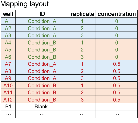
Value
A grodata object suitable to run growth.workflow. See read_data for its structure.
Examples
if(interactive()){
grodata <- parse_data(data.file = system.file("fluorescence_test_Gen5.xlsx", package = "QurvE"),
                      sheet.data = 1,
                      map.file = system.file("fluorescence_test_Gen5.xlsx", package = "QurvE"),
                      sheet.map = "mapping",
                      software = "Gen5",
                      convert.time = "y = x * 24", # convert days to hours
                      calib.growth = "y = x * 3.058") # convert absorbance to OD values
}
Extract relevant data from a raw data export file generated from the software of Perkin Elmer's "Victor Nivo" plate readers.
Description
Extract relevant data from a raw data export file generated from the software of Perkin Elmer's "Victor Nivo" plate readers.
Usage
parse_victornivo(input)
Arguments
input |
A dataframe created by reading a table file with |
Value
a list of length two containing growth and/or fluorescence dataframes in the first and second element, respectively. The first column in these dataframes represents a time vector.
Examples
if(interactive()){
input <- read_file(filename = system.file("nivo_output.csv", package = "QurvE"), csvsep = "," )
parsed <- parse_victornivo(input)
}
Extract relevant data from a raw data export file generated from the software of Perkin Elmer's "Victor X3" plate readers.
Description
Extract relevant data from a raw data export file generated from the software of Perkin Elmer's "Victor X3" plate readers.
Usage
parse_victorx3(input)
Arguments
input |
A dataframe created by reading a table file with |
Value
a list of length two containing growth and/or fluorescence dataframes in the first and second element, respectively. The first column in these dataframes represents a time vector.
Examples
if(interactive()){
input <- read_file(filename = system.file("victorx3_output.txt", package = "QurvE") )
parsed <- parse_victorx3(input)
}
Generic plot function for gcBootSpline objects.
Description
Generic plot function for gcBootSpline objects.
Usage
## S3 method for class 'drBootSpline'
plot(
  x,
  pch = 19,
  colData = 1,
  colSpline = "black",
  cex.point = 1,
  cex.lab = 1.5,
  cex.axis = 1.3,
  lwd = 2,
  plot = TRUE,
  export = FALSE,
  height = 7,
  width = 9,
  out.dir = NULL,
  combine = FALSE,
  ...
)
Arguments
x |
A |
pch |
(Numeric) Shape of the raw data symbols. |
colData |
(Numeric or Character) Color used to plot the raw data. |
colSpline |
(Numeric or Character) Color used to plot the splines. |
cex.point |
(Numeric) Size of the raw data points. |
cex.lab |
(Numeric) Font size of axis titles. |
cex.axis |
(Numeric) Font size of axis annotations. |
lwd |
(Numeric) Spline line width. |
plot |
(Logical) Show the generated plot in the |
export |
(Logical) Export the generated plot as PDF and PNG files ( |
height |
(Numeric) Height of the exported image in inches. |
width |
(Numeric) Width of the exported image in inches. |
out.dir |
(Character) Name or path to a folder in which the exported files are stored. If |
combine |
(Logical) Indicate whether both dose-response curves and parameter plots shall be shown within the same window. |
... |
Further arguments to refine the generated base R plot. |
Value
A plot with the all dose-response spline fits from the bootstrapping operation.
Examples
conc <- c(0, rev(unlist(lapply(1:18, function(x) 10*(2/3)^x))),10)
response <- c(1/(1+exp(-0.7*(4-conc[-20])))+stats::rnorm(19)/50, 0)

TestRun <- growth.drBootSpline(conc, response, drID = "test",
        control = growth.control(log.x.dr = TRUE, smooth.dr = 0.8, nboot.dr = 50))

print(summary(TestRun))
plot(TestRun, combine = TRUE)
Generic plot function for drFit objects.
Description
plot.drFit calls plot.drFitSpline for each group used in a dose-response analysis
Usage
## S3 method for class 'drFit'
plot(
  x,
  combine = TRUE,
  names = NULL,
  exclude.nm = NULL,
  pch = 16,
  cex.point = 2,
  basesize = 15,
  colors = NULL,
  lwd = 0.7,
  ec50line = TRUE,
  y.lim = NULL,
  x.lim = NULL,
  y.title = NULL,
  x.title = NULL,
  log.y = FALSE,
  log.x = FALSE,
  plot = TRUE,
  export = FALSE,
  height = NULL,
  width = NULL,
  out.dir = NULL,
  out.nm = NULL,
  ...
)
Arguments
x |
object of class |
combine |
(Logical) Combine the dose-response analysis results of all conditions into a single plot ( |
names |
(String or vector of strings) Define conditions to combine into a single plot (if |
exclude.nm |
(String or vector of strings) Define conditions to exclude from the plot (if |
pch |
(Numeric) Shape of the raw data symbols. |
cex.point |
(Numeric) Size of the raw data points. |
basesize |
(Numeric) Base font size. |
colors |
(Numeric or character) Define colors for different conditions. |
lwd |
(Numeric) Line width of the individual splines. |
ec50line |
(Logical) Show pointed horizontal and vertical lines at the EC50 values ( |
y.lim |
(Numeric vector with two elements) Optional: Provide the lower ( |
x.lim |
(Numeric vector with two elements) Optional: Provide the lower ( |
y.title |
(Character) Optional: Provide a title for the y-axis. |
x.title |
(Character) Optional: Provide a title for the x-axis. |
log.y |
(Logical) Log-transform the y-axis of the plot ( |
log.x |
(Logical) Log-transform the x-axis of the plot ( |
plot |
(Logical) Show the generated plot in the |
export |
(Logical) Export the generated plot as PDF and PNG files ( |
height |
(Numeric) Height of the exported image in inches. |
width |
(Numeric) Width of the exported image in inches. |
out.dir |
(Character) Name or path to a folder in which the exported files are stored. If |
out.nm |
(Character) The name of the PDF and PNG files if |
... |
Additional arguments. This has currently no effect and is only meant to fulfill the requirements of a generic function. |
Value
One plot per condition tested in the dose-response analysis or a single plot showing all conditions if control = growth.control(dr.method = "spline") was used in growth.drFit and combine = TRUE.
Examples
# Create random growth data set
rnd.data1 <- rdm.data(d = 35, mu = 0.8, A = 5, label = "Test1")
rnd.data2 <- rdm.data(d = 35, mu = 0.6, A = 4.5, label = "Test2")

rnd.data <- list()
rnd.data[["time"]] <- rbind(rnd.data1$time, rnd.data2$time)
rnd.data[["data"]] <- rbind(rnd.data1$data, rnd.data2$data)

# Run growth curve analysis workflow
gcFit <- growth.gcFit(time = rnd.data$time,
                       data = rnd.data$data,
                       parallelize = FALSE,
                       control = growth.control(fit.opt = "s",
                                                suppress.messages = TRUE))

# Perform dose-response analysis
drFit <- growth.drFit(gcTable = gcFit$gcTable,
                 control = growth.control(dr.parameter = "mu.spline"))

# Inspect results
summary(drFit)

plot(drFit)
Generic plot function for drFitFLModel objects.
Description
Generic plot function for drFitFLModel objects.
Usage
## S3 method for class 'drFitFLModel'
plot(
  x,
  ec50line = TRUE,
  broken = TRUE,
  bp,
  n.xbreaks,
  n.ybreaks,
  log = c("xy"),
  pch = 1,
  colSpline = 1,
  colData = 1,
  cex.point = 1,
  cex.lab = 1.5,
  cex.axis = 1.3,
  y.lim = NULL,
  x.lim = NULL,
  lwd = 2,
  plot = TRUE,
  export = FALSE,
  height = 7,
  width = 9,
  out.dir = NULL,
  ...
)
Arguments
x |
Object of class |
ec50line |
(Logical) Show pointed horizontal and vertical lines at the EC50 value ( |
broken |
(Logical) If TRUE the x axis is broken provided this axis is logarithmic (using functionality in the CRAN package 'plotrix'). |
bp |
(Numeric) Specifying the break point below which the dose is zero (the amount of stretching on the dose axis above zero in order to create the visual illusion of a logarithmic scale including 0). The default is the base-10 value corresponding to the rounded value of the minimum of the log10 values of all positive dose values. This argument is only working for logarithmic dose axes. |
n.xbreaks |
(Numeric) Number of breaks on the x-axis (if not log-transformed). The breaks are generated using |
n.ybreaks |
(Numeric) Number of breaks on the y-axis (if not log-transformed). The breaks are generated using |
log |
(Character) String which contains '"x"' if the x axis is to be logarithmic, '"y"' if the y axis is to be logarithmic and '"xy"' or '"yx"' if both axes are to be logarithmic. The default is "x". The empty string "" yields the original axes. |
pch |
(Numeric) Symbol used to plot data points. |
colSpline |
(Numeric or Character) Color used to plot the splines. |
colData |
(Numeric or Character) Color used to plot the raw data. |
cex.point |
(Numeric) Size of the raw data points. |
cex.lab |
(Numeric) Font size of axis titles. |
cex.axis |
(Numeric) Font size of axis annotations. |
y.lim |
(Numeric vector with two elements) Optional: Provide the lower ( |
x.lim |
(Numeric vector with two elements) Optional: Provide the lower ( |
lwd |
(Numeric) Line width. |
plot |
(Logical) Show the generated plot in the |
export |
(Logical) Export the generated plot as PDF and PNG files ( |
height |
(Numeric) Height of the exported image in inches. |
width |
(Numeric) Width of the exported image in inches. |
out.dir |
(Character) Name or path to a folder in which the exported files are stored. If |
... |
Further arguments to refine the generated base R plot. |
Value
A plot with the biosensor dose-response model fit.
Examples
# Create concentration values via a serial dilution
conc <- c(0, rev(unlist(lapply(1:18, function(x) 10*(2/3)^x))),10)

# Simulate response values via biosensor equation
response <- biosensor.eq(conc, y.min = 110, y.max = 6000, K = 0.5, n = 2) +
            0.01*6000*rnorm(10)

# Perform fit
TestRun <- fl.drFitModel(conc, response, drID = "test", control = fl.control())

print(summary(TestRun))
plot(TestRun)
Generic plot function for drFitModel objects.
Description
Generic plot function for drFitModel objects.
Usage
## S3 method for class 'drFitModel'
plot(
  x,
  type = c("confidence", "all", "bars", "none", "obs", "average"),
  ec50line = TRUE,
  add = FALSE,
  broken = TRUE,
  bp,
  gridsize = 200,
  log = "x",
  n.xbreaks,
  n.ybreaks,
  x.lim,
  y.lim,
  pch = 1,
  cex.point,
  cex.axis = 1,
  cex.lab = 1.3,
  col = 1,
  lwd = 2,
  lty = 2,
  xlab,
  ylab,
  legend = TRUE,
  legendText,
  legendPos,
  cex.legend = NULL,
  plot = TRUE,
  export = FALSE,
  height = 7,
  width = 9,
  out.dir = NULL,
  ...
)
Arguments
x |
object of class |
type |
(Character) Specify how to plot the data. There are currently 5 options: "average" (averages and fitted curve(s); default), "none" (only the fitted curve(s)), "obs" (only the data points), "all" (all data points and fitted curve(s)), "bars" (averages and fitted curve(s) with model-based standard errors (see Details)), and "confidence" (confidence bands for fitted curve(s)). |
ec50line |
(Logical) Show pointed horizontal and vertical lines at the EC50 values ( |
add |
(Logical) If |
broken |
(Logical) If TRUE the x axis is broken provided this axis is logarithmic (using functionality in the CRAN package 'plotrix'). |
bp |
(Numeric) Specifying the break point below which the dose is zero (the amount of stretching on the dose axis above zero in order to create the visual illusion of a logarithmic scale including 0). The default is the base-10 value corresponding to the rounded value of the minimum of the log10 values of all positive dose values. This argument is only working for logarithmic dose axes. |
gridsize |
(Numeric) Number of points in the grid used for plotting the fitted curves. |
log |
(Character) String which contains '"x"' if the x axis is to be logarithmic, '"y"' if the y axis is to be logarithmic and '"xy"' or '"yx"' if both axes are to be logarithmic. The default is "x". The empty string "" yields the original axes. |
n.xbreaks |
(Numeric) Number of breaks on the x-axis (if not log-transformed). The breaks are generated using |
n.ybreaks |
(Numeric) Number of breaks on the y-axis (if not log-transformed). The breaks are generated using |
x.lim |
(Numeric vector with two elements) Optional: Provide the lower ( |
y.lim |
(Numeric vector with two elements) Optional: Provide the lower ( |
pch |
(Numeric) Symbol used to plot data points. |
cex.point |
(Numeric) Size of the raw data points. |
cex.axis |
(Numeric) Font size of axis annotations. |
cex.lab |
(Numeric) Font size of axis titles. |
col |
(Logical or a vector of colors) If |
lwd |
(Numeric) Line width. |
lty |
(Numeric) Specify the line type. |
xlab |
(Character) An optional label for the x axis. |
ylab |
(Character) An optional label for the y axis. |
legend |
(Logical) If |
legendText |
(Character) Specify the legend text (the position of the upper right corner of the legend box). |
legendPos |
(Numeric) Vector of length 2 giving the position of the legend. |
cex.legend |
numeric specifying the legend text size. |
plot |
(Logical) Show the generated plot in the |
export |
(Logical) Export the generated plot as PDF and PNG files ( |
height |
(Numeric) Height of the exported image in inches. |
width |
(Numeric) Width of the exported image in inches. |
out.dir |
(Character) Name or path to a folder in which the exported files are stored. If |
... |
Additional arguments. This has currently no effect and is only meant to fulfill the requirements of a generic function. |
Value
A plot with the dose-response model fit.
References
Christian Ritz, Florent Baty, Jens C. Streibig, Daniel Gerhard (2015). Dose-Response Analysis Using R. PLoS ONE 10(12): e0146021. DOI: 10.1371/journal.pone.0146021
Examples
conc <- c(0, rev(unlist(lapply(1:18, function(x) 10*(2/3)^x))),10)
response <- c(1/(1+exp(-0.7*(4-conc[-20])))+stats::rnorm(19)/50, 0)

TestRun <- growth.drFitModel(conc, response, drID = "test")

print(summary(TestRun))
plot(TestRun)
Generic plot function for drFitSpline objects.
Description
plot.drFitSpline generates the spline fit plot for response-parameter vs. concentration data
Usage
## S3 method for class 'drFitSpline'
plot(
  x,
  add = FALSE,
  ec50line = TRUE,
  log = "",
  pch = 16,
  colSpline = 1,
  colData = 1,
  cex.point = 1,
  cex.lab = 1.5,
  cex.axis = 1.3,
  y.lim = NULL,
  x.lim = NULL,
  y.title = NULL,
  x.title = NULL,
  lwd = 2,
  plot = TRUE,
  export = FALSE,
  height = 7,
  width = 9,
  out.dir = NULL,
  ...
)
Arguments
x |
object of class |
add |
(Logical) Shall the fitted spline be added to an existing plot? |
ec50line |
(Logical) Show pointed horizontal and vertical lines at the EC50 value ( |
log |
("x", "y", or "xy") Display the x- or y-axis on a logarithmic scale. |
pch |
(Numeric) Shape of the raw data symbols. |
colSpline |
(Numeric or character) Spline line colour. |
colData |
(Numeric or character) Contour color of the raw data circles. |
cex.point |
(Numeric) Size of the raw data symbols. |
cex.lab |
(Numeric) Font size of axis titles. |
cex.axis |
(Numeric) Font size of axis annotations. |
y.lim |
(Numeric vector with two elements) Optional: Provide the lower ( |
x.lim |
(Numeric vector with two elements) Optional: Provide the lower ( |
y.title |
(Character) Optional: Provide a title for the y-axis. |
x.title |
(Character) Optional: Provide a title for the x-axis. |
lwd |
(Numeric) Line width of spline. |
plot |
(Logical) Show the generated plot in the |
export |
(Logical) Export the generated plot as PDF and PNG files ( |
height |
(Numeric) Height of the exported image in inches. |
width |
(Numeric) Width of the exported image in inches. |
out.dir |
(Character) Name or path to a folder in which the exported files are stored. If |
... |
Further arguments to refine the generated base R plot. |
Value
A plot with the nonparametric dose-response fit.
Examples
conc <- c(0, rev(unlist(lapply(1:18, function(x) 10*(2/3)^x))),10)
response <- c(1/(1+exp(-0.7*(4-conc[-20])))+stats::rnorm(19)/50, 0)

TestRun <- growth.drFitSpline(conc, response, drID = "test",
                     control = growth.control(log.x.dr = TRUE, smooth.dr = 0.8))

print(summary(TestRun))
plot(TestRun)
Generic plot function for drFitFL objects.
Description
drFitfl calls plot.drFitFLModel for each group used in a dose-response analysis with dr.method = "model"
Usage
## S3 method for class 'drFitfl'
plot(
  x,
  ec50line = TRUE,
  log = c("xy"),
  pch = 1,
  broken = TRUE,
  bp,
  n.xbreaks,
  n.ybreaks,
  colSpline = 1,
  colData = 1,
  cex.point = 1,
  cex.lab = 1.5,
  cex.axis = 1.3,
  y.lim = NULL,
  x.lim = NULL,
  lwd = 2,
  plot = TRUE,
  export = FALSE,
  height = 7,
  width = 9,
  out.dir = NULL,
  ...
)
Arguments
x |
object of class |
ec50line |
(Logical) Show pointed horizontal and vertical lines at the EC50 values ( |
log |
(Character) String which contains '"x"' if the x axis is to be logarithmic, '"y"' if the y axis is to be logarithmic and '"xy"' or '"yx"' if both axes are to be logarithmic. The default is "x". The empty string "" yields the original axes. |
pch |
(Numeric) Shape of the raw data symbols. |
broken |
(Logical) If TRUE the x axis is broken provided this axis is logarithmic (using functionality in the CRAN package 'plotrix'). |
bp |
(Numeric) Specifying the break point below which the dose is zero (the amount of stretching on the dose axis above zero in order to create the visual illusion of a logarithmic scale including 0). The default is the base-10 value corresponding to the rounded value of the minimum of the log10 values of all positive dose values. This argument is only working for logarithmic dose axes. |
n.xbreaks |
(Numeric) Number of breaks on the x-axis (if not log-transformed). The breaks are generated using |
n.ybreaks |
(Numeric) Number of breaks on the y-axis (if not log-transformed). The breaks are generated using |
colSpline |
(Numeric or character) Spline line colour. |
colData |
(Numeric or character) Contour color of the raw data circles. |
cex.point |
(Numeric) Size of the raw data points. |
cex.lab |
(Numeric) Font size of axis titles. |
cex.axis |
(Numeric) Font size of axis annotations. |
y.lim |
(Numeric vector with two elements) Optional: Provide the lower ( |
x.lim |
(Numeric vector with two elements) Optional: Provide the lower ( |
lwd |
(Numeric) Line width of the individual splines. |
plot |
(Logical) Show the generated plot in the |
export |
(Logical) Export the generated plot as PDF and PNG files ( |
height |
(Numeric) Height of the exported image in inches. |
width |
(Numeric) Width of the exported image in inches. |
out.dir |
(Character) Name or path to a folder in which the exported files are stored. If |
... |
Additional arguments. This has currently no effect and is only meant to fulfill the requirements of a generic function. |
Value
One plot per condition tested in the dose-response analysis (fl.drFit with control = fl.control(dr.method = "model")).
Examples
# load example dataset
input <- read_data(data.growth = system.file("lac_promoters_growth.txt", package = "QurvE"),
                   data.fl = system.file("lac_promoters_fluorescence.txt", package = "QurvE"),
                   csvsep = "\t",
                   csvsep.fl = "\t")

# Define fit controls
control <- fl.control(fit.opt = "s",
             x_type = "time", norm_fl = TRUE,
             dr.parameter = "max_slope.spline",
             dr.method = "model",
             suppress.messages = TRUE)

# Run curve fitting workflow
res <- flFit(fl_data = input$norm.fluorescence,
             time = input$time,
             parallelize = FALSE,
             control = control)

# Perform dose-response analysis with biosensor model
drFitfl <- fl.drFit(flTable = res$flTable, control = control)

plot(drFitfl)
Compare calculated dose-response parameters between conditions.
Description
plot.dr_parameter gathers parameters from the results of a dose-response analysis and compares a chosen parameter between each condition in a column plot. Error bars represent the 95% confidence interval (only shown for > 2 replicates).
Usage
## S3 method for class 'dr_parameter'
plot(
  x,
  param = c("EC50", "EC50.Estimate", "y.max", "y.min", "fc", "K", "n", "yEC50",
    "drboot.meanEC50", "drboot.meanEC50y", "EC50.orig", "yEC50.orig"),
  names = NULL,
  exclude.nm = NULL,
  basesize = 12,
  reference.nm = NULL,
  label.size = NULL,
  plot = TRUE,
  export = FALSE,
  height = 7,
  width = NULL,
  out.dir = NULL,
  out.nm = NULL,
  ...
)
Arguments
x |
A |
param |
(Character) The parameter used to compare different sample groups. Any name of a column containing numeric values in |
names |
(String or vector of strings) Define groups to combine into a single plot. Partial matches with sample/group names are accepted. If |
exclude.nm |
(String or vector of strings) Define groups to exclude from the plot. Partial matches with sample/group names are accepted. |
basesize |
(Numeric) Base font size. |
reference.nm |
(Character) Name of the reference condition, to which parameter values are normalized. Partially matching strings are tolerated as long as they can uniquely identify the condition. |
label.size |
(Numeric) Font size for sample labels below x-axis. |
plot |
(Logical) Show the generated plot in the |
export |
(Logical) Export the generated plot as PDF and PNG files ( |
height |
(Numeric) Height of the exported image in inches. |
width |
(Numeric) Width of the exported image in inches. |
out.dir |
(Character) Name or path to a folder in which the exported files are stored. If |
out.nm |
(Character) The name of the PDF and PNG files if |
... |
Additional arguments. This has currently no effect and is only meant to fulfill the requirements of a generic function. |
Value
A column plot comparing a selected parameter of a dose-response analysis between tested conditions.
Examples
# Create random growth data set
rnd.data1 <- rdm.data(d = 35, mu = 0.8, A = 5, label = "Test1")
rnd.data2 <- rdm.data(d = 35, mu = 0.6, A = 4.5, label = "Test2")

rnd.data <- list()
rnd.data[["time"]] <- rbind(rnd.data1$time, rnd.data2$time)
rnd.data[["data"]] <- rbind(rnd.data1$data, rnd.data2$data)

# Run growth curve analysis workflow
gcFit <- growth.gcFit(time = rnd.data$time,
                       data = rnd.data$data,
                       parallelize = FALSE,
                       control = growth.control(fit.opt = "s",
                                                suppress.messages = TRUE))

# Perform dose-response analysis
drFit <- growth.drFit(gcTable = gcFit$gcTable,
            control = growth.control(dr.parameter = "mu.spline"))

plot.dr_parameter(drFit, param = 'EC50')
Compare fluorescence and growth over time
Description
plot.dual creates a two-panel plot in which fluorescence or growth values are shown over time, allowing for the identification of, e.g., expression patterns in different growth stages.
Usage
## S3 method for class 'dual'
plot(
  x,
  fluorescence = c("fl", "norm.fl"),
  IDs = NULL,
  names = NULL,
  conc = NULL,
  mean = TRUE,
  exclude.nm = NULL,
  exclude.conc = NULL,
  log.y.growth = FALSE,
  log.y.fl = FALSE,
  n.ybreaks = 6,
  colors = NULL,
  color_groups = TRUE,
  group_pals = c("Green", "Orange", "Purple", "Magenta", "Grey", "Blue", "Grey", "Red",
    "Cyan", "Brown", "Mint"),
  basesize = 20,
  y.lim.growth = NULL,
  y.lim.fl = NULL,
  x.lim = NULL,
  x.title = NULL,
  y.title.growth = NULL,
  y.title.fl = NULL,
  lwd = 1.1,
  legend.position = "bottom",
  legend.ncol = 2,
  plot = TRUE,
  export = FALSE,
  height = NULL,
  width = NULL,
  out.dir = NULL,
  out.nm = NULL,
  ...
)
Arguments
x |
A |
fluorescence |
(Character) Indicate, which type of fluorescence data should be displayed. |
IDs |
(String or vector of strings) Define samples or groups (if |
names |
(String or vector of strings) Define groups to combine into a single plot. Partial matches with sample/group names are accepted. If |
conc |
(Numeric or numeric vector) Define concentrations to combine into a single plot. If |
mean |
(Logical) Display the mean and standard deviation of groups with replicates ( |
exclude.nm |
(String or vector of strings) Define groups to exclude from the plot. Partial matches with sample/group names are accepted. |
exclude.conc |
(Numeric or numeric vector) Define concentrations to exclude from the plot. |
log.y.growth |
(Logical) Log-transform the y-axis of the growth plot ( |
log.y.fl |
(Logical) Log-transform the y-axis of the fluorescence plot ( |
n.ybreaks |
(Numeric) Number of breaks on the y-axis. The breaks are generated using |
colors |
(vector of strings) Define a color palette used to draw the plots. If |
color_groups |
(Logical) Shall samples within the same group but with different concentrations be shown in different shades of the same color? |
group_pals |
(String vector) Define the colors used to display sample groups with identical concentrations. The number of selected color palettes must be at least the number of displayed groups. The order of the chosen palettes corresponds to the oder of conditions in the legend. Available options: "Green", "Oranges", "Purple", "Cyan", "Grey", "Red", "Blue", and "Magenta". |
basesize |
(Numeric) Base font size. |
y.lim.growth |
(Numeric vector with two elements) Optional: Provide the lower ( |
y.lim.fl |
(Numeric vector with two elements) Optional: Provide the lower ( |
x.lim |
(Numeric vector with two elements) Optional: Provide the lower ( |
x.title |
(Character) Optional: Provide a title for the x-axis of both growth curve and derivative plots. |
y.title.growth |
(Character) Optional: Provide a title for the y-axis of the growth plot. |
y.title.fl |
(Character) Optional: Provide a title for the y-axis of the fluorescence plot. |
lwd |
(Numeric) Line width of the individual plots. |
legend.position |
(Character) Position of the legend. One of "bottom", "top", "left", "right". |
legend.ncol |
(Numeric) Number of columns in the legend. |
plot |
(Logical) Show the generated plot in the |
export |
(Logical) Export the generated plot as PDF and PNG files ( |
height |
(Numeric) Height of the exported image in inches. |
width |
(Numeric) Width of the exported image in inches. |
out.dir |
(Character) Name or path to a folder in which the exported files are stored. If |
out.nm |
(Character) The name of the PDF and PNG files if |
... |
Additional arguments. This has currently no effect and is only meant to fulfill the requirements of a generic function. |
Value
A two-panel plot, showing raw fluorescence (fluorescence = "fl") or normalized fluorescence (fluorescence = "norm.fl") over time in the top panel, and growth over time in the bottom panel.
Examples
# load example dataset
input <- read_data(data.growth = system.file("lac_promoters_growth.txt", package = "QurvE"),
                   data.fl = system.file("lac_promoters_fluorescence.txt", package = "QurvE"),
                   csvsep = "\t",
                   csvsep.fl = "\t")

# Run workflow
res <- fl.workflow(grodata = input, ec50 = FALSE, fit.opt = "s",
                   x_type = "time", norm_fl = TRUE,
                   dr.parameter = "max_slope.spline",
                   suppress.messages = TRUE,
                   parallelize = FALSE)

plot.dual(res, legend.ncol = 3, basesize = 15)
Generic plot function for flBootSpline objects.
Description
Generic plot function for flBootSpline objects.
Usage
## S3 method for class 'flBootSpline'
plot(
  x,
  pch = 1,
  colData = 1,
  deriv = TRUE,
  colSpline = "dodgerblue3",
  cex.point = 1,
  cex.lab = 1.5,
  cex.axis = 1.3,
  lwd = 2,
  y.lim = NULL,
  x.lim = NULL,
  y.lim.deriv = NULL,
  plot = TRUE,
  export = FALSE,
  height = 7,
  width = 9,
  out.dir = NULL,
  combine = FALSE,
  ...
)
Arguments
x |
Object of class |
pch |
(Numeric) Size of the raw data circles. |
colData |
(Numeric or Character) Color used to plot the raw data. |
deriv |
(Logical) Show the derivatives (i.e., slope) over time in a secondary plot ( |
colSpline |
(Numeric or Character) Color used to plot the splines. |
cex.point |
(Numeric) Size of the raw data points. |
cex.lab |
(Numeric) Font size of axis titles. |
cex.axis |
(Numeric) Font size of axis annotations. |
lwd |
(Numeric) Spline line width. |
y.lim |
(Numeric vector with two elements) Optional: Provide the lower ( |
x.lim |
(Numeric vector with two elements) Optional: Provide the lower ( |
y.lim.deriv |
(Numeric vector with two elements) Optional: Provide the lower ( |
plot |
(Logical) Show the generated plot in the |
export |
(Logical) Export the generated plot as PDF and PNG files ( |
height |
(Numeric) Height of the exported image in inches. |
width |
(Numeric) Width of the exported image in inches. |
out.dir |
(Character) Name or path to a folder in which the exported files are stored. If |
combine |
(Logical) Indicate whether both growth curves and parameter plots shall be shown within the same window. |
... |
Additional arguments. This has currently no effect and is only meant to fulfill the requirements of a generic function. |
Value
A single plot with the all spline fits from the bootstrapping operation and statistical distribution of parameters if combine = TRUE or separate plots for fits and parameter distributions (if combine = FALSE).
Examples
# load example dataset
input <- read_data(data.growth = system.file("lac_promoters_growth.txt", package = "QurvE"),
                   data.fl = system.file("lac_promoters_fluorescence.txt", package = "QurvE"),
                   csvsep = "\t",
                   csvsep.fl = "\t")

# Extract time and normalized fluorescence data for single sample
time <- input$time[4,]
data <- input$norm.fluorescence[4,-(1:3)] # Remove identifier columns

# Perform linear fit
TestFit <- flBootSpline(time = time,
                       fl_data = data,
                       ID = "TestFit",
                       control = fl.control(fit.opt = "s", x_type = "time",
                       nboot.fl = 50))

plot(TestFit, combine = TRUE, lwd = 0.5)
Generic plot function for flcFittedLinear objects. Plot the results of a linear regression on ln-transformed data
Description
plot.flFitLinear shows the results of a linear regression and visualizes raw data, data points included in the fit, the tangent obtained by linear regression, and the lag time.
Usage
## S3 method for class 'flFitLinear'
plot(
  x,
  log = "",
  which = c("fit", "diagnostics", "fit_diagnostics"),
  pch = 21,
  cex.point = 1,
  cex.lab = 1.5,
  cex.axis = 1.3,
  lwd = 2,
  color = "firebrick3",
  y.lim = NULL,
  x.lim = NULL,
  plot = TRUE,
  export = FALSE,
  height = ifelse(which == "fit", 7, 5),
  width = ifelse(which == "fit", 9, 9),
  out.dir = NULL,
  ...
)
Arguments
x |
A |
log |
("x" or "y") Display the x- or y-axis on a logarithmic scale. |
which |
("fit" or "diagnostics") Display either the results of the linear fit on the raw data or statistical evaluation of the linear regression. |
pch |
(Numeric) Shape of the raw data symbols. |
cex.point |
(Numeric) Size of the raw data points. |
cex.lab |
(Numeric) Font size of axis titles. |
cex.axis |
(Numeric) Font size of axis annotations. |
lwd |
(Numeric) Line width. |
color |
(Character string) Enter color either by name (e.g., red, blue, coral3) or via their hexadecimal code (e.g., #AE4371, #CCFF00FF, #0066FFFF). A full list of colors available by name can be found at http://www.stat.columbia.edu/~tzheng/files/Rcolor.pdf |
y.lim |
(Numeric vector with two elements) Optional: Provide the lower ( |
x.lim |
(Numeric vector with two elements) Optional: Provide the lower ( |
plot |
(Logical) Show the generated plot in the |
export |
(Logical) Export the generated plot as PDF and PNG files ( |
height |
(Numeric) Height of the exported image in inches. |
width |
(Numeric) Width of the exported image in inches. |
out.dir |
(Character) Name or path to a folder in which the exported files are stored. If |
... |
Further arguments to refine the generated base R plot. |
Value
A plot with the linear fit.
Examples
# load example dataset
input <- read_data(data.growth = system.file("lac_promoters_growth.txt", package = "QurvE"),
                   data.fl = system.file("lac_promoters_fluorescence.txt", package = "QurvE"),
                   csvsep = "\t",
                   csvsep.fl = "\t")

# Extract time and normalized fluorescence data for single sample
time <- input$time[4,]
data <- input$norm.fluorescence[4,-(1:3)] # Remove identifier columns

# Perform linear fit
TestFit <- flFitLinear(time = time,
                       fl_data = data,
                       ID = "TestFit",
                       control = fl.control(fit.opt = "l", x_type = "time",
                       lin.R2 = 0.95, lin.RSD = 0.1,
                       lin.h = 20))

plot(TestFit)
Combine different groups of samples into a single plot
Description
Visualize fluorescence, normalized fluorescence, or spline fits of multiple sample groups in a single plot.
Usage
## S3 method for class 'flFitRes'
plot(
  x,
  data.type = c("spline", "raw", "norm.fl"),
  IDs = NULL,
  names = NULL,
  conc = NULL,
  mean = TRUE,
  exclude.nm = NULL,
  exclude.conc = NULL,
  log.y = FALSE,
  deriv = FALSE,
  n.ybreaks = 6,
  colors = NULL,
  color_groups = TRUE,
  group_pals = c("Green", "Orange", "Purple", "Magenta", "Grey", "Blue", "Grey", "Red",
    "Cyan", "Brown", "Mint"),
  basesize = 20,
  y.lim = NULL,
  x.lim = NULL,
  y.title = NULL,
  x.title = NULL,
  y.lim.deriv = NULL,
  y.title.deriv = NULL,
  lwd = 1.1,
  legend.position = "bottom",
  legend.ncol = 2,
  plot = TRUE,
  export = FALSE,
  height = NULL,
  width = NULL,
  out.dir = NULL,
  out.nm = NULL,
  ...
)

## S3 method for class 'flFit'
plot(
  x,
  data.type = c("spline", "raw", "norm.fl"),
  IDs = NULL,
  names = NULL,
  conc = NULL,
  mean = TRUE,
  exclude.nm = NULL,
  exclude.conc = NULL,
  log.y = FALSE,
  deriv = FALSE,
  n.ybreaks = 6,
  colors = NULL,
  color_groups = TRUE,
  group_pals = c("Green", "Orange", "Purple", "Magenta", "Grey", "Blue", "Grey", "Red",
    "Cyan", "Brown", "Mint"),
  basesize = 20,
  y.lim = NULL,
  x.lim = NULL,
  y.title = NULL,
  x.title = NULL,
  y.lim.deriv = NULL,
  y.title.deriv = NULL,
  lwd = 1.1,
  legend.position = "bottom",
  legend.ncol = 2,
  plot = TRUE,
  export = FALSE,
  height = NULL,
  width = NULL,
  out.dir = NULL,
  out.nm = NULL,
  ...
)
Arguments
x |
A |
data.type |
(Character) Indicate, which type of fluorescence data should be displayed. |
IDs |
(String or vector of strings) Define samples or groups (if |
names |
(String or vector of strings) Define groups to combine into a single plot. Partial matches with sample/group names are accepted. If |
conc |
(Numeric or numeric vector) Define concentrations to combine into a single plot. If |
mean |
(Logical) Display the mean and standard deviation of groups with replicates ( |
exclude.nm |
(String or vector of strings) Define groups to exclude from the plot. Partial matches with sample/group names are accepted. |
exclude.conc |
(Numeric or numeric vector) Define concentrations to exclude from the plot. |
log.y |
(Logical) Log-transform the y-axis of the plot ( |
deriv |
(Logical) Show derivatives over time in a separate panel below the plot ( |
n.ybreaks |
(Numeric) Number of breaks on the y-axis. The breaks are generated using |
colors |
(vector of strings) Define a color palette used to draw the plots. If |
color_groups |
(Logical) Shall samples within the same group but with different concentrations be shown in different shades of the same color? |
group_pals |
(String vector) Define the colors used to display sample groups with identical concentrations. The number of selected color palettes must be at least the number of displayed groups. The order of the chosen palettes corresponds to the oder of conditions in the legend. Available options: "Green", "Oranges", "Purple", "Cyan", "Grey", "Red", "Blue", and "Magenta". |
basesize |
(Numeric) Base font size. |
y.lim |
(Numeric vector with two elements) Optional: Provide the lower ( |
x.lim |
(Numeric vector with two elements) Optional: Provide the lower ( |
y.title |
(Character) Optional: Provide a title for the y-axis of the fluorescence curve plot. |
x.title |
(Character) Optional: Provide a title for the x-axis of both fluorescence curve and derivative plots. |
y.lim.deriv |
(Numeric vector with two elements) Optional: Provide the lower ( |
y.title.deriv |
(Character) Optional: Provide a title for the y-axis of the derivative plot. |
lwd |
(Numeric) Line width of the individual plots. |
legend.position |
(Character) Position of the legend. One of "bottom", "top", "left", "right". |
legend.ncol |
(Numeric) Number of columns in the legend. |
plot |
(Logical) Show the generated plot in the |
export |
(Logical) Export the generated plot as PDF and PNG files ( |
height |
(Numeric) Height of the exported image in inches. |
width |
(Numeric) Width of the exported image in inches. |
out.dir |
(Character) Name or path to a folder in which the exported files are stored. If |
out.nm |
(Character) The name of the PDF and PNG files if |
... |
Additional arguments. This has currently no effect and is only meant to fulfill the requirements of a generic function. |
Value
A plot with all curves (nonparametric fits, raw fluorescence measurements, or raw normalized fluorescence over time) in a flFitRes object created with fl.workflow, with replicates combined by the group averages (if mean = TRUE) or not (mean = FALSE).
A plot with all curves (raw fluorescence measurements or raw normalized fluorescence over time) in a flFit object with flFit, with replicates combined by the group averages (if mean = TRUE) or not (mean = FALSE).
Examples
# load example dataset
input <- read_data(data.growth = system.file("lac_promoters_growth.txt", package = "QurvE"),
                   data.fl = system.file("lac_promoters_fluorescence.txt", package = "QurvE"),
                   csvsep = "\t",
                   csvsep.fl = "\t")

# Run workflow
res <- fl.workflow(grodata = input, ec50 = FALSE, fit.opt = "s",
                   x_type = "time", norm_fl = TRUE,
                   dr.parameter = "max_slope.spline",
                   suppress.messages = TRUE,
                   parallelize = FALSE)

plot(res, legend.ncol = 3, basesize = 15)


# load example dataset
input <- read_data(data.growth = system.file("lac_promoters_growth.txt", package = "QurvE"),
                   data.fl = system.file("lac_promoters_fluorescence.txt", package = "QurvE"),
                   csvsep = "\t",
                   csvsep.fl = "\t")

# Run curve fitting workflow
res <- flFit(fl_data = input$norm.fluorescence,
             time = input$time,
             parallelize = FALSE,
             control = fl.control(fit.opt = "s", suppress.messages = TRUE,
             x_type = "time", norm_fl = TRUE))

plot(res, legend.ncol = 3, basesize = 15)
Generic plot function for flFitSpline objects.
Description
plot.flFitSpline generates the spline fit plot for a single sample.
Usage
## S3 method for class 'flFitSpline'
plot(
  x,
  add = FALSE,
  raw = TRUE,
  slope = TRUE,
  deriv = TRUE,
  spline = TRUE,
  log.y = FALSE,
  basesize = 16,
  pch = 1,
  colData = 1,
  colSpline = "dodgerblue3",
  cex.point = 2,
  lwd = 0.7,
  y.lim = NULL,
  x.lim = NULL,
  y.lim.deriv = NULL,
  n.ybreaks = 6,
  y.title = NULL,
  x.title = NULL,
  y.title.deriv = NULL,
  plot = TRUE,
  export = FALSE,
  width = 8,
  height = ifelse(deriv == TRUE, 8, 6),
  out.dir = NULL,
  ...
)
Arguments
x |
Object of class |
add |
(Logical) Shall the fitted spline be added to an existing plot? |
raw |
(Logical) Display raw growth as circles ( |
slope |
(Logical) Show the slope at the maximum slope ( |
deriv |
(Logical) Show the derivative (i.e., slope) over time in a secondary plot ( |
spline |
(Logical) Only for |
log.y |
(Logical) Log-transform the y-axis ( |
basesize |
(Numeric) Base font size. |
pch |
(Numeric) Symbol used to plot data points. |
colData |
(Numeric or character) Contour color of the raw data circles. |
colSpline |
(Numeric or character) Spline line colour. |
cex.point |
(Numeric) Size of the raw data points. |
lwd |
(Numeric) Spline line width. |
y.lim |
(Numeric vector with two elements) Optional: Provide the lower ( |
x.lim |
(Numeric vector with two elements) Optional: Provide the lower ( |
y.lim.deriv |
(Numeric vector with two elements) Optional: Provide the lower ( |
n.ybreaks |
(Numeric) Number of breaks on the y-axis. The breaks are generated using |
y.title |
(Character) Optional: Provide a title for the y-axis of the growth curve plot. |
x.title |
(Character) Optional: Provide a title for the x-axis of both growth curve and derivative plots. |
y.title.deriv |
(Character) Optional: Provide a title for the y-axis of the derivative plot. |
plot |
(Logical) Show the generated plot in the |
export |
(Logical) Export the generated plot as PDF and PNG files ( |
width |
(Numeric) Width of the exported image in inches. |
height |
(Numeric) Height of the exported image in inches. |
out.dir |
(Character) Name or path to a folder in which the exported files are stored. If |
... |
Additional arguments. This has currently no effect and is only meant to fulfill the requirements of a generic function. |
Value
A plot with the nonparametric fit.
Examples
# load example dataset
input <- read_data(data.growth = system.file("lac_promoters_growth.txt", package = "QurvE"),
                   data.fl = system.file("lac_promoters_fluorescence.txt", package = "QurvE"),
                   csvsep = "\t",
                   csvsep.fl = "\t")

# Extract time and normalized fluorescence data for single sample
time <- input$time[4,]
data <- input$norm.fluorescence[4,-(1:3)] # Remove identifier columns

# Perform linear fit
TestFit <- flFitSpline(time = time,
                       fl_data = data,
                       ID = "TestFit",
                       control = fl.control(fit.opt = "s", x_type = "time"))

plot(TestFit)
Generic plot function for gcBootSpline objects.
Description
Generic plot function for gcBootSpline objects.
Usage
## S3 method for class 'gcBootSpline'
plot(
  x,
  pch = 1,
  colData = 1,
  deriv = TRUE,
  colSpline = "dodgerblue3",
  cex.point = 1,
  cex.lab = 1.5,
  cex.axis = 1.3,
  lwd = 2,
  y.lim = NULL,
  x.lim = NULL,
  y.lim.deriv = NULL,
  plot = TRUE,
  export = FALSE,
  height = 7,
  width = 9,
  out.dir = NULL,
  combine = FALSE,
  ...
)
Arguments
x |
object of class |
pch |
(Numeric) Symbol used to plot data points. |
colData |
(Numeric or character) Contour color of the raw data circles. |
deriv |
(Logical) Show the derivatives (i.e., slope) over time in a secondary plot ( |
colSpline |
(Numeric or character) Spline line colour. |
cex.point |
(Numeric) Size of the raw data points. |
cex.lab |
(Numeric) Font size of axis titles. |
cex.axis |
(Numeric) Font size of axis annotations. |
lwd |
(Numeric) Spline line width. |
y.lim |
(Numeric vector with two elements) Optional: Provide the lower ( |
x.lim |
(Numeric vector with two elements) Optional: Provide the lower ( |
y.lim.deriv |
(Numeric vector with two elements) Optional: Provide the lower ( |
plot |
(Logical) Show the generated plot in the |
export |
(Logical) Export the generated plot as PDF and PNG files ( |
height |
(Numeric) Height of the exported image in inches. |
width |
(Numeric) Width of the exported image in inches. |
out.dir |
(Character) Name or path to a folder in which the exported files are stored. If |
combine |
(Logical) Indicate whether both growth curves and parameter plots shall be shown within the same window. |
... |
Further arguments to refine the generated base R plot. |
Value
A single plot with the all spline growth fits from the bootstrapping operation and statistical distribution of growth parameters if combine = TRUE or separate plots for growth fits and parameter distributions (if combine = FALSE).
Examples
# Create random growth dataset
rnd.dataset <- rdm.data(d = 35, mu = 0.8, A = 5, label = "Test1")

# Extract time and growth data for single sample
time <- rnd.dataset$time[1,]
data <- rnd.dataset$data[1,-(1:3)] # Remove identifier columns

# Introduce some noise into the measurements
data <- data + stats::runif(97, -0.01, 0.09)

# Perform bootstrapping spline fit
TestFit <- growth.gcBootSpline(time, data, gcID = "TestFit",
              control = growth.control(fit.opt = "s", nboot.gc = 50))

plot(TestFit, combine = TRUE, lwd = 0.5)
Generic plot function for gcFittedLinear objects. Plot the results of a linear regression on ln-transformed data
Description
plot.gcFitLinear shows the results of a linear regression on log-transformed data and visualizes raw data, data points included in the fit, the tangent obtained by linear regression, and the lag time.
Usage
## S3 method for class 'gcFitLinear'
plot(
  x,
  log = "y",
  which = c("fit", "diagnostics", "fit_diagnostics"),
  pch = 21,
  cex.point = 1,
  cex.lab = 1.5,
  cex.axis = 1.3,
  lwd = 2,
  color = "firebrick3",
  y.lim = NULL,
  x.lim = NULL,
  plot = TRUE,
  export = FALSE,
  height = ifelse(which == "fit", 7, 5),
  width = ifelse(which == "fit", 9, 9),
  out.dir = NULL,
  ...
)
Arguments
x |
A |
log |
("x" or "y") Display the x- or y-axis on a logarithmic scale. |
which |
("fit" or "diagnostics") Display either the results of the linear fit on the raw data or statistical evaluation of the linear regression. |
pch |
(Numeric) Shape of the raw data symbols. |
cex.point |
(Numeric) Size of the raw data points. |
cex.lab |
(Numeric) Font size of axis titles. |
cex.axis |
(Numeric) Font size of axis annotations. |
lwd |
(Numeric) Line width. |
color |
(Character string) Enter color either by name (e.g., red, blue, coral3) or via their hexadecimal code (e.g., #AE4371, #CCFF00FF, #0066FFFF). A full list of colors available by name can be found at http://www.stat.columbia.edu/~tzheng/files/Rcolor.pdf |
y.lim |
(Numeric vector with two elements) Optional: Provide the lower ( |
x.lim |
(Numeric vector with two elements) Optional: Provide the lower ( |
plot |
(Logical) Show the generated plot in the |
export |
(Logical) Export the generated plot as PDF and PNG files ( |
height |
(Numeric) Height of the exported image in inches. |
width |
(Numeric) Width of the exported image in inches. |
out.dir |
(Character) Name or path to a folder in which the exported files are stored. If |
... |
Further arguments to refine the generated base R plot. |
Value
A plot with the linear fit.
Examples
# Create random growth dataset
rnd.dataset <- rdm.data(d = 35, mu = 0.8, A = 5, label = "Test1")

# Extract time and growth data for single sample
time <- rnd.dataset$time[1,]
data <- rnd.dataset$data[1,-(1:3)] # Remove identifier columns

# Perform linear fit
TestFit <- growth.gcFitLinear(time, data, gcID = "TestFit",
                 control = growth.control(fit.opt = "l"))

plot(TestFit)
Generic plot function for gcFitModel objects.
Description
Plot the results of a parametric model fit on growth vs. time data
Usage
## S3 method for class 'gcFitModel'
plot(
  x,
  raw = TRUE,
  pch = 1,
  colData = 1,
  equation = TRUE,
  eq.size = 1,
  colModel = "forestgreen",
  basesize = 16,
  cex.point = 2,
  lwd = 0.7,
  x.lim = NULL,
  y.lim = NULL,
  n.ybreaks = 6,
  plot = TRUE,
  export = FALSE,
  height = 6,
  width = 8,
  out.dir = NULL,
  ...
)
Arguments
x |
A |
raw |
(Logical) Show the raw data within the plot ( |
pch |
(Numeric) Symbol used to plot data points. |
colData |
(Numeric or Character) Color used to plot the raw data. |
equation |
(Logical) Show the equation of the fitted model within the plot ( |
eq.size |
(Numeric) Provide a value to scale the size of the displayed equation. |
colModel |
(Numeric or Character) Color used to plot the fitted model. |
basesize |
(Numeric) Base font size. |
cex.point |
(Numeric) Size of the raw data points. |
lwd |
(Numeric) Spline line width. |
x.lim |
(Numeric vector with two elements) Optional: Provide the lower ( |
y.lim |
(Numeric vector with two elements) Optional: Provide the lower ( |
n.ybreaks |
(Numeric) Number of breaks on the y-axis. The breaks are generated using |
plot |
(Logical) Show the generated plot in the |
export |
(Logical) Export the generated plot as PDF and PNG files ( |
height |
(Numeric) Height of the exported image in inches. |
width |
(Numeric) Width of the exported image in inches. |
out.dir |
(Character) Name or path to a folder in which the exported files are stored. If |
... |
Further arguments to refine the generated |
Value
A plot with the parametric fit.
Examples
# Create random growth dataset
rnd.dataset <- rdm.data(d = 35, mu = 0.8, A = 5, label = "Test1")

# Extract time and growth data for single sample
time <- rnd.dataset$time[1,]
data <- rnd.dataset$data[1,-(1:3)] # Remove identifier columns

# Perform parametric fit
TestFit <- growth.gcFitModel(time, data, gcID = "TestFit",
                 control = growth.control(fit.opt = "m"))

plot(TestFit, basesize = 18, eq.size = 1.5)
Generic plot function for gcFitSpline objects.
Description
plot.gcFitSpline generates the spline fit plot for a single sample.
Usage
## S3 method for class 'gcFitSpline'
plot(
  x,
  add = FALSE,
  raw = TRUE,
  slope = TRUE,
  deriv = TRUE,
  spline = TRUE,
  log.y = TRUE,
  pch = 1,
  colData = 1,
  colSpline = "dodgerblue3",
  basesize = 16,
  cex.point = 2,
  lwd = 0.7,
  y.lim = NULL,
  x.lim = NULL,
  y.lim.deriv = NULL,
  n.ybreaks = 6,
  y.title = NULL,
  x.title = NULL,
  y.title.deriv = NULL,
  plot = TRUE,
  export = FALSE,
  width = 8,
  height = ifelse(deriv == TRUE, 8, 6),
  out.dir = NULL,
  ...
)
Arguments
x |
object of class |
add |
(Logical) Shall the fitted spline be added to an existing plot? |
raw |
(Logical) Display raw growth as circles ( |
slope |
(Logical) Show the slope at the maximum growth rate ( |
deriv |
(Logical) Show the derivative (i.e., slope) over time in a secondary plot ( |
spline |
(Logical) Only for |
log.y |
(Logical) Log-transform the y-axis ( |
pch |
(Numeric) Symbol used to plot data points. |
colData |
(Numeric or character) Contour color of the raw data circles. |
colSpline |
(Numeric or character) Spline line colour. |
basesize |
(Numeric) Base font size. |
cex.point |
(Numeric) Size of the raw data points. |
lwd |
(Numeric) Spline line width. |
y.lim |
(Numeric vector with two elements) Optional: Provide the lower ( |
x.lim |
(Numeric vector with two elements) Optional: Provide the lower ( |
y.lim.deriv |
(Numeric vector with two elements) Optional: Provide the lower ( |
n.ybreaks |
(Numeric) Number of breaks on the y-axis. The breaks are generated using |
y.title |
(Character) Optional: Provide a title for the y-axis of the growth curve plot. |
x.title |
(Character) Optional: Provide a title for the x-axis of both growth curve and derivative plots. |
y.title.deriv |
(Character) Optional: Provide a title for the y-axis of the derivative plot. |
plot |
(Logical) Show the generated plot in the |
export |
(Logical) Export the generated plot as PDF and PNG files ( |
width |
(Numeric) Width of the exported image in inches. |
height |
(Numeric) Height of the exported image in inches. |
out.dir |
(Character) Name or path to a folder in which the exported files are stored. If |
... |
Further arguments to refine the generated base R plot (if |
Value
A plot with the nonparametric fit.
Examples
# Create random growth dataset
rnd.dataset <- rdm.data(d = 35, mu = 0.8, A = 5, label = "Test1")

# Extract time and growth data for single sample
time <- rnd.dataset$time[1,]
data <- rnd.dataset$data[1,-(1:3)] # Remove identifier columns

# Perform spline fit
TestFit <- growth.gcFitSpline(time, data, gcID = "TestFit",
                 control = growth.control(fit.opt = "s"))

plot(TestFit)
Plot a matrix of growth curve panels
Description
plot.grid takes a grofit or flFitRes object and returns a facet grid of individual growth and fluorescence plots
Usage
## S3 method for class 'grid'
plot(
  x,
  data.type = c("spline", "raw", "norm.fl"),
  param = c("mu.linfit", "lambda.linfit", "dY.linfit", "A.linfit", "mu2.linfit",
    "lambda2.linfit", "mu.model", "lambda.model", "A.model", "A.orig.model", "dY.model",
    "dY.orig.model", "tD.linfit", "tD2.linfit", "tD.spline", "tD2.spline", "mu.spline",
    "lambda.spline", "A.spline", "dY.spline", "integral.spline", "mu2.spline",
    "lambda2.spline", "mu.bt", "lambda.bt", "A.bt", "integral.bt", "max_slope.linfit",
    "max_slope.spline"),
  pal = c("Green", "Orange", "Purple", "Magenta", "Grey", "Blue", "Grey", "Red", "Cyan",
    "Brown", "Mint"),
  invert.pal = FALSE,
  IDs = NULL,
  sort_by_ID = FALSE,
  names = NULL,
  conc = NULL,
  exclude.nm = NULL,
  exclude.conc = NULL,
  mean = TRUE,
  log.y = TRUE,
  n.ybreaks = 6,
  sort_by_conc = TRUE,
  nrow = NULL,
  basesize = 20,
  y.lim = NULL,
  x.lim = NULL,
  legend.lim = NULL,
  y.title = NULL,
  x.title = NULL,
  lwd = 1.1,
  plot = TRUE,
  export = FALSE,
  height = NULL,
  width = NULL,
  out.dir = NULL,
  out.nm = NULL,
  ...
)
Arguments
x |
A |
data.type |
(Character) Plot either raw data ( |
param |
(Character) The parameter used to compare different sample groups. Any name of a column containing numeric values in |
pal |
(Character string) Choose one of 'Green', 'Orange', 'Purple', 'Magenta', 'Grey', 'Blue', 'Grey', 'Red', 'Cyan', 'Brown', or 'Mint' to visualize the value of the parameter chosen as |
invert.pal |
(Logical) Shall the colors in the chosen |
IDs |
(String or vector of strings) Define samples or groups (if |
sort_by_ID |
(Logical) Shall samples/conditions be ordered as entered in |
names |
(String or vector of strings) Define groups to combine into a single plot. Partial matches with sample/group names are accepted. If |
conc |
(Numeric or numeric vector) Define concentrations to combine into a single plot. If |
exclude.nm |
(String or vector of strings) Define groups to exclude from the plot. Partial matches with sample/group names are accepted. |
exclude.conc |
(Numeric or numeric vector) Define concentrations to exclude from the plot. |
mean |
(Logical) Display the mean and standard deviation of groups with replicates ( |
log.y |
(Logical) Log-transform the y-axis of the plot ( |
n.ybreaks |
(Numeric) Number of breaks on the y-axis. The breaks are generated using |
sort_by_conc |
(Logical) Shall the samples/conditions be sorted with concentrations in rows and groups in columns? |
nrow |
(Numeric) Defines the number of rows in the grid if |
basesize |
(Numeric) Base font size. |
y.lim |
(Numeric vector with two elements) Optional: Provide the lower ( |
x.lim |
(Numeric vector with two elements) Optional: Provide the lower ( |
legend.lim |
(Numeric vector with two elements) Optional: Provide the lower ( |
y.title |
(Character) Optional: Provide a title for the y-axis of the growth curve plot. |
x.title |
(Character) Optional: Provide a title for the x-axis of both growth curve and derivative plots. |
lwd |
(Numeric) Line width of the individual plots. |
plot |
(Logical) Show the generated plot in the |
export |
(Logical) Export the generated plot as PDF and PNG files ( |
height |
(Numeric) Height of the exported image in inches. |
width |
(Numeric) Width of the exported image in inches. |
out.dir |
(Character) Name or path to a folder in which the exported files are stored. If |
out.nm |
(Character) The name of the PDF and PNG files if |
... |
Additional arguments. This has currently no effect and is only meant to fulfill the requirements of a generic function. |
Value
A plot matrix with all growth curves (raw measurements or nonparametric fits) in a dataset, with replicates combined by the group averages (if mean = TRUE) or not (mean = FALSE).
Examples
# Create random growth data set
rnd.data1 <- rdm.data(d = 35, mu = 0.8, A = 5, label = "Test1")
rnd.data2 <- rdm.data(d = 35, mu = 0.6, A = 4.5, label = "Test2")

rnd.data <- list()
rnd.data[["time"]] <- rbind(rnd.data1$time, rnd.data2$time)
rnd.data[["data"]] <- rbind(rnd.data1$data, rnd.data2$data)

# Run growth curve analysis workflow
res <- growth.workflow(time = rnd.data$time,
                       data = rnd.data$data,
                       fit.opt = "s",
                       ec50 = FALSE,
                       export.res = FALSE,
                       suppress.messages = TRUE,
                       parallelize = FALSE)


plot.grid(res, param = "mu.spline")
Generic plot function for grodata objects. Plots raw growth, fluorescence, or normalized fluorescence data of multiple samples or conditions.
Description
plot.grodata calls plot.grofit or plot.flFitRes based on the chosen data.type, respectively.
Usage
## S3 method for class 'grodata'
plot(
  x,
  data.type = c("growth", "fl", "norm.fl"),
  IDs = NULL,
  names = NULL,
  conc = NULL,
  mean = TRUE,
  exclude.nm = NULL,
  exclude.conc = NULL,
  log.y = FALSE,
  n.ybreaks = 6,
  colors = NULL,
  color_groups = TRUE,
  group_pals = c("Green", "Orange", "Purple", "Magenta", "Grey", "Blue", "Grey", "Red",
    "Cyan", "Brown", "Mint"),
  basesize = 20,
  y.lim = NULL,
  x.lim = NULL,
  y.title = NULL,
  x.title = NULL,
  lwd = 1.1,
  legend.position = "bottom",
  legend.ncol = 2,
  plot = TRUE,
  export = FALSE,
  height = NULL,
  width = NULL,
  out.dir = NULL,
  out.nm = NULL,
  ...
)
Arguments
x |
A |
data.type |
(Character) Plot either raw growth ( |
IDs |
(String or vector of strings) Define samples or groups (if |
names |
(String or vector of strings) Define groups to combine into a single plot. Partial matches with sample/group names are accepted. If |
conc |
(Numeric or numeric vector) Define concentrations to combine into a single plot. If |
mean |
(Logical) Display the mean and standard deviation of groups with replicates ( |
exclude.nm |
(String or vector of strings) Define groups to exclude from the plot. Partial matches with sample/group names are accepted. |
exclude.conc |
(Numeric or numeric vector) Define concentrations to exclude from the plot. |
log.y |
(Logical) Log-transform the y-axis of the plot ( |
n.ybreaks |
(Numeric) Number of breaks on the y-axis. The breaks are generated using |
colors |
(vector of strings) Define a color palette used to draw the plots. If |
color_groups |
(Logical) Shall samples within the same group but with different concentrations be shown in different shades of the same color? |
group_pals |
(String vector) Define the colors used to display sample groups with identical concentrations. The number of selected color palettes must be at least the number of displayed groups. The order of the chosen palettes corresponds to the oder of conditions in the legend. Available options: "Green", "Oranges", "Purple", "Cyan", "Grey", "Red", "Blue", and "Magenta". |
basesize |
(Numeric) Base font size. |
y.lim |
(Numeric vector with two elements) Optional: Provide the lower ( |
x.lim |
(Numeric vector with two elements) Optional: Provide the lower ( |
y.title |
(Character) Optional: Provide a title for the y-axis of the growth curve plot. |
x.title |
(Character) Optional: Provide a title for the x-axis of both growth curve and derivative plots. |
lwd |
(Numeric) Line width of the individual plots. |
legend.position |
(Character) Position of the legend. One of "bottom", "top", "left", "right". |
legend.ncol |
(Numeric) Number of columns in the legend. |
plot |
(Logical) Show the generated plot in the |
export |
(Logical) Export the generated plot as PDF and PNG files ( |
height |
(Numeric) Height of the exported image in inches. |
width |
(Numeric) Width of the exported image in inches. |
out.dir |
(Character) Name or path to a folder in which the exported files are stored. If |
out.nm |
(Character) The name of the PDF and PNG files if |
... |
Additional arguments. This has currently no effect and is only meant to fulfill the requirements of a generic function. |
Value
A plot with all growth curves (raw measurements) in a dataset, with replicates combined by the group averages (if mean = TRUE) or not (mean = FALSE).
Examples
# Create random growth data sets
rnd.data1 <- rdm.data(d = 35, mu = 0.8, A = 5, label = "Test1")
rnd.data2 <- rdm.data(d = 35, mu = 0.6, A = 4.5, label = "Test2")

# Create dataframe with both data sets and a single time vector
time <- as.data.frame(matrix(t(c("Time",NA,NA, rnd.data1$time[1,])),nrow=1),
             stringsAsFactors=FALSE)
colnames(time) <- colnames(rnd.data1$data)
data <- rbind(time, rnd.data1$data, rnd.data2$data)


# Create a grodata object
grodata <- read_data(data.growth = data, data.format = "row")

plot(grodata, exclude.nm = "Test1", legend.ncol = 4)
Generic plot function for grofit objects. Combine different groups of samples into a single plot
Description
plot.grofit extracts the spline fits of a subset of samples in a grofit object calculates averages and standard deviations of conditions with replicates and combines them into a single plot.
Usage
## S3 method for class 'grofit'
plot(
  x,
  ...,
  data.type = c("spline", "raw"),
  IDs = NULL,
  names = NULL,
  conc = NULL,
  exclude.nm = NULL,
  exclude.conc = NULL,
  mean = TRUE,
  log.y = TRUE,
  deriv = TRUE,
  n.ybreaks = 6,
  colors = NULL,
  color_groups = TRUE,
  group_pals = c("Green", "Orange", "Purple", "Magenta", "Grey", "Blue", "Grey", "Red",
    "Cyan", "Brown", "Mint"),
  basesize = 20,
  y.lim = NULL,
  x.lim = NULL,
  y.title = NULL,
  x.title = NULL,
  y.lim.deriv = NULL,
  y.title.deriv = NULL,
  lwd = 1.1,
  legend.position = "bottom",
  legend.ncol = 2,
  plot = TRUE,
  export = FALSE,
  height = NULL,
  width = NULL,
  out.dir = NULL,
  out.nm = NULL
)
Arguments
x |
A |
... |
(optional) Additional |
data.type |
(Character) Plot either raw data ( |
IDs |
(String or vector of strings) Define samples or groups (if |
names |
(String or vector of strings) Define groups to combine into a single plot. Partial matches with sample/group names are accepted. If |
conc |
(Numeric or numeric vector) Define concentrations to combine into a single plot. If |
exclude.nm |
(String or vector of strings) Define groups to exclude from the plot. Partial matches with sample/group names are accepted. |
exclude.conc |
(Numeric or numeric vector) Define concentrations to exclude from the plot. |
mean |
(Logical) Display the mean and standard deviation of groups with replicates ( |
log.y |
(Logical) Log-transform the y-axis of the plot ( |
deriv |
(Logical) Show derivatives over time in a separate panel below the plot ( |
n.ybreaks |
(Numeric) Number of breaks on the y-axis. The breaks are generated using |
colors |
(vector of strings) Define a color palette used to draw the plots. If |
color_groups |
(Logical) Shall samples within the same group but with different concentrations be shown in different shades of the same color? |
group_pals |
(String vector) Define the colors used to display sample groups with identical concentrations. The number of selected color palettes must be at least the number of displayed groups. The order of the chosen palettes corresponds to the oder of conditions in the legend. Available options: "Green", "Oranges", "Purple", "Cyan", "Grey", "Red", "Blue", and "Magenta". |
basesize |
(Numeric) Base font size. |
y.lim |
(Numeric vector with two elements) Optional: Provide the lower ( |
x.lim |
(Numeric vector with two elements) Optional: Provide the lower ( |
y.title |
(Character) Optional: Provide a title for the y-axis of the growth curve plot. |
x.title |
(Character) Optional: Provide a title for the x-axis of both growth curve and derivative plots. |
y.lim.deriv |
(Numeric vector with two elements) Optional: Provide the lower ( |
y.title.deriv |
(Character) Optional: Provide a title for the y-axis of the derivative plot. |
lwd |
(Numeric) Line width of the individual plots. |
legend.position |
(Character) Position of the legend. One of "bottom", "top", "left", "right". |
legend.ncol |
(Numeric) Number of columns in the legend. |
plot |
(Logical) Show the generated plot in the |
export |
(Logical) Export the generated plot as PDF and PNG files ( |
height |
(Numeric) Height of the exported image in inches. |
width |
(Numeric) Width of the exported image in inches. |
out.dir |
(Character) Name or path to a folder in which the exported files are stored. If |
out.nm |
(Character) The name of the PDF and PNG files if |
Value
A plot with all growth curves (raw measurements or nonparametric fits) in a dataset, with replicates combined by the group averages (if mean = TRUE) or not (mean = FALSE).
Examples
# Create random growth data set
rnd.data1 <- rdm.data(d = 35, mu = 0.8, A = 5, label = "Test1")
rnd.data2 <- rdm.data(d = 35, mu = 0.6, A = 4.5, label = "Test2")

rnd.data <- list()
rnd.data[["time"]] <- rbind(rnd.data1$time, rnd.data2$time)
rnd.data[["data"]] <- rbind(rnd.data1$data, rnd.data2$data)

# Run growth curve analysis workflow
res <- growth.workflow(time = rnd.data$time,
                       data = rnd.data$data,
                       fit.opt = "s",
                       ec50 = FALSE,
                       export.res = FALSE,
                       suppress.messages = TRUE,
                       parallelize = FALSE)


plot(res, names = "Test1", legend.ncol = 4) # Show only samples for condition "Test1"
Compare growth parameters between samples or conditions
Description
plot.parameter gathers physiological parameters from the results of a growth fit analysis and compares a chosen parameter between each sample or condition in a column plot. Error bars represent the 95% confidence interval (only shown for > 2 replicates).
Usage
## S3 method for class 'parameter'
plot(
  x,
  param = c("mu.linfit", "lambda.linfit", "dY.linfit", "A.linfit", "mu2.linfit",
    "lambda2.linfit", "mu.model", "lambda.model", "A.model", "A.orig.model", "dY.model",
    "dY.orig.model", "tD.linfit", "tD2.linfit", "tD.spline", "tD2.spline", "mu.spline",
    "lambda.spline", "A.spline", "dY.spline", "integral.spline", "mu2.spline",
    "lambda2.spline", "mu.bt", "lambda.bt", "A.bt", "integral.bt", "max_slope.linfit",
    "max_slope.spline"),
  IDs = NULL,
  names = NULL,
  conc = NULL,
  exclude.nm = NULL,
  exclude.conc = NULL,
  reference.nm = NULL,
  reference.conc = NULL,
  order_by_conc = FALSE,
  colors = NULL,
  basesize = 12,
  label.size = NULL,
  shape.size = 2.5,
  legend.position = "right",
  legend.ncol = 1,
  plot = TRUE,
  export = FALSE,
  height = 7,
  width = NULL,
  out.dir = NULL,
  out.nm = NULL,
  ...
)
Arguments
x |
A |
param |
(Character) The parameter used to compare different sample groups. Any name of a column containing numeric values in |
IDs |
(String or vector of strings) Define samples or groups (if |
names |
(String or vector of strings) Define groups to combine into a single plot. Partial matches with sample/group names are accepted. If |
conc |
(Numeric or numeric vector) Define concentrations to combine into a single plot. If |
exclude.nm |
(String or vector of strings) Define groups to exclude from the plot. Partial matches with sample/group names are accepted. |
exclude.conc |
(Numeric or numeric vector) Define concentrations to exclude from the plot. |
reference.nm |
(Character) Name of the reference condition, to which parameter values are normalized. Partially matching strings are tolerated as long as they can uniquely identify the condition. |
reference.conc |
(Numeric) Concentration of the reference condition, to which parameter values are normalized. |
order_by_conc |
(Logical) Shall the columns be sorted in order of ascending concentrations ( |
colors |
(vector of strings) Define a color palette used to draw the columns. If |
basesize |
(Numeric) Base font size. |
label.size |
(Numeric) Font size for sample labels below x-axis. |
shape.size |
(Numeric) The size of the symbols indicating replicate values. Default: 2.5 |
legend.position |
(Character) Position of the legend. One of "bottom", "top", "left", "right". |
legend.ncol |
(Numeric) Number of columns in the legend. |
plot |
(Logical) Show the generated plot in the |
export |
(Logical) Export the generated plot as PDF and PNG files ( |
height |
(Numeric) Height of the exported image in inches. |
width |
(Numeric) Width of the exported image in inches. |
out.dir |
(Character) Name or path to a folder in which the exported files are stored. If |
out.nm |
(Character) The name of the PDF and PNG files if |
... |
Additional arguments. This has currently no effect and is only meant to fulfill the requirements of a generic function. |
Value
A column plot comparing a selected growth parameter between tested conditions.
Examples
# Create random growth data set
rnd.data1 <- rdm.data(d = 35, mu = 0.8, A = 5, label = "Test1")
rnd.data2 <- rdm.data(d = 35, mu = 0.6, A = 4.5, label = "Test2")

rnd.data <- list()
rnd.data[["time"]] <- rbind(rnd.data1$time, rnd.data2$time)
rnd.data[["data"]] <- rbind(rnd.data1$data, rnd.data2$data)

# Run growth curve analysis workflow
res <- growth.workflow(time = rnd.data$time,
                       data = rnd.data$data,
                       fit.opt = "s",
                       ec50 = FALSE,
                       export.res = FALSE,
                       parallelize = FALSE,
                       suppress.messages = TRUE)


plot.parameter(res,
               param = "mu.spline",
               legend.ncol = 4,
               legend.position = "bottom",
               basesize = 15,
               label.size = 11)
The function calls the baranyi function to generate curves between time zero and t and adds some random noise to the x- and y-axes. The three growth parameters given as input values will be slightly changed to produce different growth curves. The resulting datasets can be used to test the growth.workflow function.
Description
The function calls the baranyi function to generate curves between time zero and t and adds some random noise to the x- and y-axes. The three growth parameters given as input values will be slightly changed to produce different growth curves. The resulting datasets can be used to test the growth.workflow function.
Usage
rdm.data(d, y0 = 0.05, tmax = 24, mu = 0.6, lambda = 5, A = 3, label = "Test1")
Arguments
d |
Numeric value, number of data sets. If |
y0 |
Numeric value, start growth. If |
tmax |
Numeric value, number of time points per data set. If |
mu |
Numeric value, maximum slope. If |
lambda |
Numeric value, lag-phase. If |
A |
Numeric value, maximum growth. If |
label |
Character string, condition label If |
Value
A list containing simulated data for three tests (e.g., 'organisms'):
time |
numeric matrix of size |
data |
data.frame of size |
References
Matthias Kahm, Guido Hasenbrink, Hella Lichtenberg-Frate, Jost Ludwig, Maik Kschischo (2010). grofit: Fitting Biological Growth Curves with R. Journal of Statistical Software, 33(7), 1-21. DOI: 10.18637/jss.v033.i07
Examples
# Create random growth data set
rnd.data1 <- rdm.data(d = 35, mu = 0.8, A = 5, label = 'Test1')
rnd.data2 <- rdm.data(d = 35, mu = 0.6, A = 4.5, label = 'Test2')

rnd.data <- list()
rnd.data[['time']] <- rbind(rnd.data1$time, rnd.data2$time)
rnd.data[['data']] <- rbind(rnd.data1$data, rnd.data2$data)

# Run growth curve analysis workflow
gcFit <- growth.gcFit(time = rnd.data$time,
                       data = rnd.data$data,
                       parallelize = FALSE,
                       control = growth.control(fit.opt = 's',
                                                suppress.messages = TRUE))


# Perform dose-response analysis
drFit <- growth.drFit(gcTable = gcFit$gcTable,
             control = growth.control(dr.parameter = 'mu.spline'))

# Inspect results
summary(drFit)
plot(drFit)
Read growth and fluorescence data in table format
Description
read_data reads table files or R dataframe objects containing growth and fluorescence data and extracts datasets, sample and group information, performs blank correction, applies data transformation (calibration), and combines technical replicates.
Usage
read_data(
  data.growth = NA,
  data.fl = NA,
  data.fl2 = NA,
  data.format = "col",
  csvsep = ";",
  dec = ".",
  csvsep.fl = ";",
  dec.fl = ".",
  csvsep.fl2 = ";",
  dec.fl2 = ".",
  sheet.growth = 1,
  sheet.fl = 1,
  sheet.fl2 = 1,
  fl.normtype = c("growth", "fl2"),
  subtract.blank = TRUE,
  convert.time = NULL,
  calib.growth = NULL,
  calib.fl = NULL,
  calib.fl2 = NULL
)
Arguments
data.growth |
An R dataframe object or a table file with extension '.xlsx', '.xls', '.csv', '.tsv', or '.txt' containing growth data. The data must be either in the '
Data in 'tidy' format requires the following column headers:
|
data.fl |
(optional) An R dataframe object or a table file with extension '.xlsx', '.xls', '.csv', '.tsv', or '.txt' containing fluorescence data. Table layout must mimic that of |
data.fl2 |
(optional) An R dataframe object or a table file with extension '.xlsx', '.xls', '.csv', '.tsv', or '.txt' containing measurements from a second fluorescence channel (used only to normalize |
data.format |
(Character) "col" for samples in columns, or "row" for samples in rows. Default: |
csvsep |
(Character) separator used in CSV file storing growth data (ignored for other file types). Default: |
dec |
(Character) decimal separator used in CSV, TSV or TXT file storing growth data. Default: |
csvsep.fl, csvsep.fl2 |
(Character) separator used in CSV file storing fluorescence data (ignored for other file types). Default: |
dec.fl, dec.fl2 |
(Character) decimal separator used in CSV, TSV or TXT file storing fluorescence data. Default: |
sheet.growth, sheet.fl, sheet.fl2 |
(Numeric or Character) Number or name of the sheet with the respective data type in XLS or XLSX files (optional). |
fl.normtype |
(Character string) Normalize fluorescence values by either diving by |
subtract.blank |
(Logical) Shall blank values be subtracted from values within the same experiment (TRUE, the default) or not (FALSE). |
convert.time |
( |
calib.growth, calib.fl, calib.fl2 |
(Character or |
Details
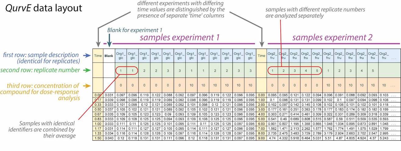
Value
An R list object of class grodata containing a time matrix, dataframes with growth and fluorescence data (if applicable),
and an experimental design table. The grodata object can be directly
used to run growth.workflow/fl.workflow or, together with a growth.control/fl.control
object, in growth.gcFit/flFit.
time |
Matrix with raw time values extracted from |
growth |
Dataframe with raw growth values and sample identifiers extracted from |
fluorescence |
Dataframe with raw fluorescence values and sample identifiers extracted from |
norm.fluorescence |
fluorescence data divided by growth values. |
expdesign |
Experimental design table created from the first three identifier rows/columns (see argument |
Examples
# Load CSV file containing only growth data
data_growth <- read_data(data.growth = system.file("2-FMA_toxicity.csv",
                         package = "QurvE"), csvsep = ";" )

# Load XLS file containing both growth and fluorescence data
data_growth_fl <- read_data(
                    data.growth = system.file("lac_promoters_growth.txt", package = "QurvE"),
                    data.fl = system.file("lac_promoters_fluorescence.txt", package = "QurvE"),
                    csvsep = "\t",
                    csvsep.fl = "\t")
Call the appropriate function required to read a table file and return the table as a dataframe object.
Description
read_file automatically detects the format of a file provided as filename and calls the appropriate function to read the table file.
Usage
read_file(filename, csvsep = ";", dec = ".", sheet = 1)
Arguments
filename |
(Character) Name or path of the table file to read. Can be of type CSV, XLS, XLSX, TSV, or TXT. |
csvsep |
(Character) separator used in CSV file (ignored for other file types). |
dec |
(Character) decimal separator used in CSV, TSV and TXT files. |
sheet |
(Numeric or Character) Number or name of a sheet in XLS or XLSX files (optional). Default: |
Value
A dataframe object with headers in the first row.
Examples
input <- read_file(filename = system.file("2-FMA_toxicity.csv", package = "QurvE"), csvsep = ";" )
Run Shiny QurvE App
Description
Run Shiny QurvE App
Usage
run_app()
Value
Launches a browser with the shiny app
Examples
if(interactive()){
# Run the app
run_app()
}
Single hue palettes for ggplot2
Description
These palettes are used in the package for plotting.
Usage
single_hue_palettes
Format
An object of class list of length 11.
Generic summary function for drBootSpline objects
Description
Generic summary function for drBootSpline objects
Usage
## S3 method for class 'drBootSpline'
summary(object, ...)
Arguments
object |
object of class |
... |
Additional arguments. This has currently no effect and is only meant to fulfill the requirements of a generic function. |
Value
A dataframe with statistical parameters extracted from the dose-response bootstrapping analysis.
Examples
conc <- c(0, rev(unlist(lapply(1:18, function(x) 10*(2/3)^x))),10)
response <- c(1/(1+exp(-0.7*(4-conc[-20])))+stats::rnorm(19)/50, 0)

TestRun <- growth.drBootSpline(conc, response, drID = 'test',
        control = growth.control(log.x.dr = TRUE, smooth.dr = 0.8, nboot.dr = 50))

print(summary(TestRun))
Generic summary function for drFit objects
Description
Generic summary function for drFit objects
Usage
## S3 method for class 'drFit'
summary(object, ...)
Arguments
object |
object of class |
... |
Additional arguments. This has currently no effect and is only meant to fulfill the requirements of a generic function. |
Value
A dataframe with parameters for all samples extracted from the dose-response analysis.
Examples
# Create random growth data set
rnd.data1 <- rdm.data(d = 35, mu = 0.8, A = 5, label = 'Test1')
rnd.data2 <- rdm.data(d = 35, mu = 0.6, A = 4.5, label = 'Test2')

rnd.data <- list()
rnd.data[['time']] <- rbind(rnd.data1$time, rnd.data2$time)
rnd.data[['data']] <- rbind(rnd.data1$data, rnd.data2$data)

# Run growth curve analysis workflow
gcFit <- growth.gcFit(time = rnd.data$time,
                       data = rnd.data$data,
                       parallelize = FALSE,
                       control = growth.control(fit.opt = 's',
                                                suppress.messages = TRUE))

# Perform dose-response analysis
drFit <- growth.drFit(gcTable = gcFit$gcTable,
                 control = growth.control(dr.parameter = 'mu.spline'))

# Inspect results
summary(drFit)
Generic summary function for drFitFLModel objects
Description
Generic summary function for drFitFLModel objects
Usage
## S3 method for class 'drFitFLModel'
summary(object, ...)
Arguments
object |
object of class |
... |
Additional arguments. This has currently no effect and is only meant to fulfill the requirements of a generic function. |
Value
A dataframe with biosensor response parameters.
Examples
# Create concentration values via a serial dilution
conc <- c(0, rev(unlist(lapply(1:18, function(x) 10*(2/3)^x))),10)

# Simulate response values via biosensor equation
response <- biosensor.eq(conc, y.min = 110, y.max = 6000, K = 0.5, n = 2) +
            0.01*6000*rnorm(10)

# Perform fit
TestRun <- fl.drFitModel(conc, response, drID = 'test', control = fl.control())

print(summary(TestRun))
Generic summary function for drFitModel objects
Description
Generic summary function for drFitModel objects
Usage
## S3 method for class 'drFitModel'
summary(object, ...)
Arguments
object |
object of class |
... |
Additional arguments. This has currently no effect and is only meant to fulfill the requirements of a generic function. |
Value
A dataframe with parameters extracted from the dose-response analysis of a single sample.
Examples
conc <- c(0, rev(unlist(lapply(1:18, function(x) 10*(2/3)^x))),10)
response <- c(1/(1+exp(-0.7*(4-conc[-20])))+rnorm(19)/50, 0)

TestRun <- growth.drFitModel(conc, response, drID = 'test')

print(summary(TestRun))
Generic summary function for drFitSpline objects
Description
Generic summary function for drFitSpline objects
Usage
## S3 method for class 'drFitSpline'
summary(object, ...)
Arguments
object |
object of class |
... |
Additional arguments. This has currently no effect and is only meant to fulfill the requirements of a generic function. |
Value
A dataframe with parameters extracted from the dose-response analysis of a single sample.
Examples
conc <- c(0, rev(unlist(lapply(1:18, function(x) 10*(2/3)^x))),10)
response <- c(1/(1+exp(-0.7*(4-conc[-20])))+rnorm(19)/50, 0)

TestRun <- growth.drFitSpline(conc, response, drID = 'test',
              control = growth.control(log.x.dr = TRUE, smooth.dr = 0.8))

print(summary(TestRun))
Generic summary function for drFitfl objects
Description
Generic summary function for drFitfl objects
Usage
## S3 method for class 'drFitfl'
summary(object, ...)
Arguments
object |
object of class |
... |
Additional arguments. This has currently no effect and is only meant to fulfill the requirements of a generic function. |
Value
A dataframe with parameters for all samples extracted from a dose-response analysis.
Examples
# load example dataset
input <- read_data(data.growth = system.file("lac_promoters_growth.txt", package = "QurvE"),
                   data.fl = system.file("lac_promoters_fluorescence.txt", package = "QurvE"),
                   csvsep = "\t",
                   csvsep.fl = "\t")

# Define fit controls
control <- fl.control(fit.opt = 's',
             x_type = 'time', norm_fl = TRUE,
             dr.parameter = 'max_slope.spline',
             dr.method = 'model',
             suppress.messages = TRUE)

# Run curve fitting workflow
res <- flFit(fl_data = input$norm.fluorescence,
             time = input$time,
             parallelize = FALSE,
             control = control)

# Perform dose-response analysis with biosensor model
drFitfl <- fl.drFit(flTable = res$flTable, control = control)

summary(drFitfl)
Generic summary function for flBootSpline objects
Description
Generic summary function for flBootSpline objects
Usage
## S3 method for class 'flBootSpline'
summary(object, ...)
Arguments
object |
object of class |
... |
Additional arguments. This has currently no effect and is only meant to fulfill the requirements of a generic function. |
Value
A dataframe with statistical parameters extracted from a dose-response bootstrapping analysis.
Examples
# load example dataset
input <- read_data(data.growth = system.file("lac_promoters_growth.txt", package = "QurvE"),
                   data.fl = system.file("lac_promoters_fluorescence.txt", package = "QurvE"),
                   csvsep = "\t",
                   csvsep.fl = "\t")

# Extract time and normalized fluorescence data for single sample
time <- input$time[4,]
data <- input$norm.fluorescence[4,-(1:3)] # Remove identifier columns

# Perform linear fit
TestFit <- flBootSpline(time = time,
                       fl_data = data,
                       ID = 'TestFit',
                       control = fl.control(fit.opt = 's', x_type = 'time',
                       nboot.fl = 50))

summary(TestFit)
Generic summary function for flFit objects
Description
Generic summary function for flFit objects
Usage
## S3 method for class 'flFit'
summary(object, ...)
Arguments
object |
object of class |
... |
Additional arguments. This has currently no effect and is only meant to fulfill the requirements of a generic function. |
Value
A dataframe with parameters extracted from all fits of a workflow.
Examples
# load example dataset
input <- read_data(data.growth = system.file("lac_promoters_growth.txt", package = "QurvE"),
                   data.fl = system.file("lac_promoters_fluorescence.txt", package = "QurvE"),
                   csvsep = "\t",
                   csvsep.fl = "\t")

# Run curve fitting workflow
res <- flFit(fl_data = input$norm.fluorescence,
             time = input$time,
             parallelize = FALSE,
             control = fl.control(fit.opt = 's', suppress.messages = TRUE,
             x_type = 'time', norm_fl = TRUE, nboot.fl = 20))

summary(res)
Generic summary function for flFitLinear objects
Description
Generic summary function for flFitLinear objects
Usage
## S3 method for class 'flFitLinear'
summary(object, ...)
Arguments
object |
object of class |
... |
Additional arguments. This has currently no effect and is only meant to fulfill the requirements of a generic function. |
Value
A dataframe with parameters extracted from a linear fit.
Examples
# load example dataset
input <- read_data(data.growth = system.file("lac_promoters_growth.txt", package = "QurvE"),
                   data.fl = system.file("lac_promoters_fluorescence.txt", package = "QurvE"),
                   csvsep = "\t",
                   csvsep.fl = "\t")

# Extract time and normalized fluorescence data for single sample
time <- input$time[4,]
data <- input$norm.fluorescence[4,-(1:3)] # Remove identifier columns

# Perform linear fit
TestFit <- flFitLinear(time = time,
                       fl_data = data,
                       ID = 'TestFit',
                       control = fl.control(fit.opt = 'l', x_type = 'time',
                       lin.R2 = 0.95, lin.RSD = 0.1,
                       lin.h = 20))

summary(TestFit)
Generic summary function for flFitSpline objects
Description
Generic summary function for flFitSpline objects
Usage
## S3 method for class 'flFitSpline'
summary(object, ...)
Arguments
object |
object of class |
... |
Additional arguments. This has currently no effect and is only meant to fulfill the requirements of a generic function. |
Value
A dataframe with parameters extracted from a nonparametric fit.
Examples
# load example dataset
input <- read_data(data.growth = system.file("lac_promoters_growth.txt", package = "QurvE"),
                   data.fl = system.file("lac_promoters_fluorescence.txt", package = "QurvE"),
                   csvsep = "\t",
                   csvsep.fl = "\t")

# Extract time and normalized fluorescence data for single sample
time <- input$time[4,]
data <- input$norm.fluorescence[4,-(1:3)] # Remove identifier columns

# Perform linear fit
TestFit <- flFitSpline(time = time,
                       fl_data = data,
                       ID = 'TestFit',
                       control = fl.control(fit.opt = 's', x_type = 'time'))

summary(TestFit)
Generic summary function for gcBootSpline objects
Description
Generic summary function for gcBootSpline objects
Usage
## S3 method for class 'gcBootSpline'
summary(object, ...)
Arguments
object |
object of class |
... |
Additional arguments. This has currently no effect and is only meant to fulfill the requirements of a generic function. |
Value
A dataframe with statistical parameters extracted from the spline fit bootstrapping computation.
Examples
# Create random growth dataset
rnd.dataset <- rdm.data(d = 35, mu = 0.8, A = 5, label = 'Test1')

# Extract time and growth data for single sample
time <- rnd.dataset$time[1,]
data <- rnd.dataset$data[1,-(1:3)] # Remove identifier columns

# Introduce some noise into the measurements
data <- data + stats::runif(97, -0.01, 0.09)

# Perform bootstrapping spline fit
TestFit <- growth.gcBootSpline(time, data, gcID = 'TestFit',
              control = growth.control(fit.opt = 's', nboot.gc = 50))

summary(TestFit)
Generic summary function for gcFit objects
Description
Generic summary function for gcFit objects
Usage
## S3 method for class 'gcFit'
summary(object, ...)
Arguments
object |
object of class |
... |
Additional arguments. This has currently no effect and is only meant to fulfill the requirements of a generic function. |
Value
A dataframe with parameters extracted from all fits of a workflow.
Examples
# Create random growth data set
rnd.data1 <- rdm.data(d = 35, mu = 0.8, A = 5, label = 'Test1')
rnd.data2 <- rdm.data(d = 35, mu = 0.6, A = 4.5, label = 'Test2')

rnd.data <- list()
rnd.data[['time']] <- rbind(rnd.data1$time, rnd.data2$time)
rnd.data[['data']] <- rbind(rnd.data1$data, rnd.data2$data)

# Run growth curve analysis workflow
gcFit <- growth.gcFit(time = rnd.data$time,
                       data = rnd.data$data,
                       parallelize = FALSE,
                       control = growth.control(fit.opt = 's',
                                                suppress.messages = TRUE,
                                                nboot.gc = 20))
summary(gcFit)
Generic summary function for gcFitLinear objects
Description
Generic summary function for gcFitLinear objects
Usage
## S3 method for class 'gcFitLinear'
summary(object, ...)
Arguments
object |
object of class |
... |
Additional arguments. This has currently no effect and is only meant to fulfill the requirements of a generic function. |
Value
A dataframe with parameters extracted from the linear fit.
Examples
# Create random growth dataset
rnd.dataset <- rdm.data(d = 35, mu = 0.8, A = 5, label = 'Test1')

# Extract time and growth data for single sample
time <- rnd.dataset$time[1,]
data <- rnd.dataset$data[1,-(1:3)] # Remove identifier columns

# Perform linear fit
TestFit <- growth.gcFitLinear(time, data, gcID = 'TestFit',
                 control = growth.control(fit.opt = 'l'))

summary(TestFit)
Generic summary function for gcFitModel objects
Description
Generic summary function for gcFitModel objects
Usage
## S3 method for class 'gcFitModel'
summary(object, ...)
Arguments
object |
object of class |
... |
Additional arguments. This has currently no effect and is only meant to fulfill the requirements of a generic function. |
Value
A dataframe with parameters extracted from the growth model fit.
Examples
# Create random growth dataset
rnd.dataset <- rdm.data(d = 35, mu = 0.8, A = 5, label = 'Test1')

# Extract time and growth data for single sample
time <- rnd.dataset$time[1,]
data <- rnd.dataset$data[1,-(1:3)] # Remove identifier columns

# Perform parametric fit
TestFit <- growth.gcFitModel(time, data, gcID = 'TestFit',
                 control = growth.control(fit.opt = 'm'))

summary(TestFit)
Generic summary function for gcFitSpline objects
Description
Generic summary function for gcFitSpline objects
Usage
## S3 method for class 'gcFitSpline'
summary(object, ...)
Arguments
object |
object of class |
... |
Additional arguments. This has currently no effect and is only meant to fulfill the requirements of a generic function. |
Value
A dataframe with parameters extracted from the nonparametric fit.
Examples
# Create random growth dataset
rnd.dataset <- rdm.data(d = 35, mu = 0.8, A = 5, label = 'Test1')

# Extract time and growth data for single sample
time <- rnd.dataset$time[1,]
data <- rnd.dataset$data[1,-(1:3)] # Remove identifier columns

# Perform linear fit
TestFit <- growth.gcFitSpline(time, data, gcID = 'TestFit',
                 control = growth.control(fit.opt = 's'))

summary(TestFit)
Generate a grouped results table for linear fits with average and standard deviations
Description
Generate a grouped results table for linear fits with average and standard deviations
Usage
table_group_fluorescence_linear(flTable, html = FALSE)
Arguments
flTable |
An object of class |
html |
(Logical) Should column headers contain html formatting? |
Value
A data frame with grouped linear fit results. Empty cells indicate that no reliable fit could be determined.
Examples
# load example dataset
input <- read_data(data.growth = system.file("lac_promoters_growth.txt", package = "QurvE"),
                   data.fl = system.file("lac_promoters_fluorescence.txt", package = "QurvE"),
                   csvsep = "\t",
                   csvsep.fl = "\t")

# Run workflow
res <- fl.workflow(grodata = input, ec50 = FALSE, fit.opt = "l",
                   x_type = "time", norm_fl = TRUE,
                   dr.parameter = "max_slope.spline",
                   suppress.messages = TRUE,
                   parallelize = FALSE)

table_group_fluorescence_linear(res$flFit$flTable)

# with HTML formatting
DT::datatable(table_group_fluorescence_linear(res$flFit$flTable, html = TRUE),
              escape = FALSE) # Do not escape HTML entities
Generate a grouped results table for spline fits with average and standard deviations
Description
Generate a grouped results table for spline fits with average and standard deviations
Usage
table_group_fluorescence_spline(flTable, html = FALSE)
Arguments
flTable |
An object of class |
html |
(Logical) Should column headers contain html formatting? |
Value
A data frame with grouped spline fit results. Empty cells indicate that no reliable fit could be determined.
Examples
# load example dataset
input <- read_data(data.growth = system.file("lac_promoters_growth.txt", package = "QurvE"),
                   data.fl = system.file("lac_promoters_fluorescence.txt", package = "QurvE"),
                   csvsep = "\t",
                   csvsep.fl = "\t")

# Run workflow
res <- fl.workflow(grodata = input, ec50 = FALSE, fit.opt = "s",
                   x_type = "time", norm_fl = TRUE,
                   dr.parameter = "max_slope.spline",
                   suppress.messages = TRUE,
                   parallelize = FALSE)

table_group_fluorescence_spline(res$flFit$flTable)

# with HTML formatting
DT::datatable(table_group_fluorescence_spline(res$flFit$flTable, html = TRUE),
              escape = FALSE) # Do not escape HTML entities
Generate a grouped results table for linear fits with average and standard deviations
Description
Generate a grouped results table for linear fits with average and standard deviations
Usage
table_group_growth_linear(gcTable, html = FALSE)
Arguments
gcTable |
An object of class |
html |
(Logical) Should column headers contain html formatting? |
Value
A data frame with grouped linear fit results. Empty cells indicate that no reliable fit could be determined.
Examples
# Create random growth data set
rnd.data <- rdm.data(d = 30, mu = 0.6, A = 4.5, label = "Test2")


# Run growth curve analysis workflow
res <- growth.workflow(time = rnd.data$time,
                       data = rnd.data$data,
                       fit.opt = "l",
                       ec50 = FALSE,
                       export.res = FALSE,
                       parallelize = FALSE,
                       suppress.messages = TRUE)

table_group_growth_linear(res$gcFit$gcTable)

# with HTML formatting
DT::datatable(table_group_growth_linear(res$gcFit$gcTable, html = TRUE),
              escape = FALSE) # Do not escape HTML entities
Generate a grouped results table for parametric fits with average and standard deviations
Description
Generate a grouped results table for parametric fits with average and standard deviations
Usage
table_group_growth_model(gcTable, html = FALSE)
Arguments
gcTable |
An object of class |
html |
(Logical) Should column headers contain html formatting? |
Value
A data frame with grouped model fit results. Empty cells indicate that no reliable fit could be determined.
Examples
# Create random growth data set
rnd.data <- rdm.data(d = 35, mu = 0.8, A = 5, label = "Test1")


# Run growth curve analysis workflow
res <- growth.workflow(time = rnd.data$time,
                       data = rnd.data$data,
                       fit.opt = "m",
                       ec50 = FALSE,
                       export.res = FALSE,
                       parallelize = FALSE,
                       suppress.messages = TRUE)

table_group_growth_model(res$gcFit$gcTable)

# with HTML formatting
DT::datatable(table_group_growth_model(res$gcFit$gcTable, html = TRUE),
              escape = FALSE) # Do not escape HTML entities
Generate a grouped results table for spline fits with average and standard deviations
Description
Generate a grouped results table for spline fits with average and standard deviations
Usage
table_group_growth_spline(gcTable, html = FALSE)
Arguments
gcTable |
An object of class |
html |
(Logical) Should column headers contain html formatting? |
Value
A data frame with grouped spline fit results. Empty cells indicate that no reliable fit could be determined.
Examples
# Create random growth data set
rnd.data <- rdm.data(d = 35, mu = 0.8, A = 5, label = "Test1")

# Run growth curve analysis workflow
res <- growth.workflow(time = rnd.data$time,
                       data = rnd.data$data,
                       fit.opt = "s",
                       ec50 = FALSE,
                       export.res = FALSE,
                       parallelize = FALSE,
                       suppress.messages = TRUE)

table_group_growth_spline(res$gcFit$gcTable)

# with HTML formatting
DT::datatable(table_group_growth_spline(res$gcFit$gcTable, html = TRUE),
              escape = FALSE) # Do not escape HTML entities
Convert a tidy data frame to a custom QurvE format
Description
This function converts a data frame in "tidy" format into the custom format used by QurvE (row format).
The provided "tidy" data has columns for "Description", "Concentration", "Replicate", and "Values", with one
row per time point and sample. Alternatively, the function converts data in custom QurvE column format into
row format (if data.format = "col").
Usage
tidy_to_custom(df, data.format = "col")
Arguments
df |
A data frame in tidy format, containing "Time", "Description", and either "Values" or "Value" columns. Optionally, meta information provided in columns "Replicate" and "Concentration" is used. |
data.format |
(Character string) |
Value
A data frame in the custom format (row format) used by QurvE.
Examples
# Create a tidy data frame with two samples, five concentrations, three
# replicates, and five time points
samples <- c("Sample 1", "Sample 2")
concentrations <- c(0.1, 0.5, 1, 2, 5)
time_points <- c(1, 2, 3, 4, 5)
n_replicates <- 3

df <- expand.grid(
   Description = c("Sample 1", "Sample 2"),
   Concentration = c(0.1, 0.5, 1, 2, 5),
   Time = c(1, 2, 3, 4, 5),
   Replicate = 1:3)

df$Value <- abs(rnorm(nrow(df)))

df_formatted <- tidy_to_custom(df)
Create an update-resistant popover for a Shiny element
Description
This function creates a popover that is resistant to updates in the associated Shiny element. It adds an event listener to the specified element, which reinstalls the popover whenever a child of the element changes.
Usage
updateResistantPopover(
  id,
  title,
  content,
  placement = "bottom",
  trigger = "hover",
  options = NULL
)
Arguments
id |
The id of the Shiny element to which the popover is attached. |
title |
The title of the popover. |
content |
The content of the popover. |
placement |
The placement of the popover relative to the Shiny element (default: "bottom"). Possible values are "top", "bottom", "left", and "right". |
trigger |
The event that triggers the display of the popover (default: "hover"). Possible values are "hover", "focus", and "click". |
options |
A list of additional options for the popover. |
Value
A Shiny HTML tag that contains the JavaScript code for creating the update-resistant popover.
Author(s)
K. Rohde (stack overflow)
Examples
## Not run:
library(shiny)
library(shinyBS)

ui <- shinyUI(fluidPage(
  selectInput("Main2_1","Label","abc",  selectize = TRUE, multiple = TRUE),
  updateResistantPopover("Main2_1", "Label", "content", placement = "right", trigger = "focus"),
  actionButton("destroy", "destroy!")
))

server <- function(input, output, session){
  observeEvent(input$destroy, {
    updateSelectInput(session, "Main2_1", choices="foo")
  })
}

shinyApp(ui, server)

## End(Not run)
Combine two dataframes like a zip-fastener
Description
Combine rows or columns of two dataframes in an alternating manner
Usage
zipFastener(df1, df2, along = 2)
Arguments
df1 |
A first dataframe. |
df2 |
A second dataframe with the same dimensions as |
along |
|
Value
A dataframe with combined rows (or columns) of df1 and df2.
Author(s)
Mark Heckmann
Examples
# data frames equal dimensions
df1 <- plyr::rdply(3, rep('o',4))[ ,-1]
df2 <- plyr::rdply(3, rep('X',4))[ ,-1]

zipFastener(df1, df2)
zipFastener(df1, df2, 2)
zipFastener(df1, df2, 1)

# data frames unequal in no. of rows
df1 <- plyr::rdply(10, rep('o',4))[ ,-1]
zipFastener(df1, df2, 1)
zipFastener(df2, df1, 1)

# data frames unequal in no. of columns
df2 <- plyr::rdply(10, rep('X',3))[ ,-1]
zipFastener(df1, df2)
zipFastener(df2, df1, 2)