| Type: | Package |
| Title: | Spatial KWD for Large Spatial Maps |
| Version: | 0.4.1 |
| Date: | 2022-12-09 |
| Author: | Stefano Gualandi [aut, cre] |
| Maintainer: | Stefano Gualandi <stefano.gualandi@gmail.com> |
| Description: | Contains efficient implementations of Discrete Optimal Transport algorithms for the computation of Kantorovich-Wasserstein distances between pairs of large spatial maps (Bassetti, Gualandi, Veneroni (2020), <doi:10.1137/19M1261195>). All the algorithms are based on an ad-hoc implementation of the Network Simplex algorithm. The package has four main helper functions: compareOneToOne() (to compare two spatial maps), compareOneToMany() (to compare a reference map with a list of other maps), compareAll() (to compute a matrix of distances between a list of maps), and focusArea() (to compute the KWD distance within a focus area). In non-convex maps, the helper functions first build the convex-hull of the input bins and pad the weights with zeros. |
| License: | EUPL (≥ 1.2) |
| Imports: | methods, Rcpp |
| SystemRequirements: | C++11 |
| LinkingTo: | Rcpp |
| NeedsCompilation: | yes |
| Packaged: | 2022-12-09 16:21:03 UTC; stegua |
| Repository: | CRAN |
| Date/Publication: | 2022-12-09 17:00:02 UTC |
Kantorovich-Wasserstein Distances for Large Spatial Maps
Description
The Spatial-KWD package contains efficient implementations of Discrete Optimal Transport algorithms for the computation of Kantorovich-Wasserstein distances [1], customized for large spatial maps. All the algorithms are based on an ad-hoc implementation of the Network Simplex algorithm [2]. Each implemented algorithm builds a different network, exploiting the particular structure of spatial maps.
Details
This library contains four helper functions and two classes [4].
The four helper functions are compareOneToOne, compareOneToMany, compareAll, and focusArea. All the functions take in input the data and an options list. Using the options is possible to configure the Kantorivich-Wasserstein solver, so that it uses different algorithms with different parameters.
The helper functions are built on top of two main classes: Histogram2D and Solver.
Note that in non-convex maps, the algorithm builds the convex-hull of the input bins and pads the weights with zeros.
In the case of spatial histograms with weights that do not sum up to 1, all the weights can optionally be rescaled in such a way the overall sum of the weights of every single histogram is equal to 1.0: w_i \gets \frac{w_i}{\sum_{i=1,\dots,n} w_i}.
This way, the spatial histograms have a natural interpretation as discrete probability measures.
For a detailed introduction on Computational Optimal Transport, we refer the reader to [3].
Author(s)
Stefano Gualandi, stefano.gualandi@gmail.com.
Maintainer: Stefano Gualandi <stefano.gualandi@gmail.com>
References
[1] Bassetti, F., Gualandi, S. and Veneroni, M., 2020. "On the Computation of Kantorovich–Wasserstein Distances Between Two-Dimensional Histograms by Uncapacitated Minimum Cost Flows". SIAM Journal on Optimization, 30(3), pp.2441-2469.
[2] Cunningham, W.H., 1976. "A Network Simplex method". Mathematical Programming, 11(1), pp.105-116.
[3] Peyre, G., and Cuturi, M., 2019. "Computational optimal transport: With applications to data science". Foundations and Trends in Machine Learning, 11(5-6), pp.355-607.
[4] https://github.com/eurostat/Spatial-KWD
See Also
See also compareOneToOne, compareOneToMany, compareAll, focusArea, Histogram2D, and Solver.
Examples
library(SpatialKWD)

# Random coordinates
N = 90
Xs <- as.integer(runif(N, 0, 31))
Ys <- as.integer(runif(N, 0, 31))
coordinates <- matrix(c(Xs, Ys), ncol=2)

# Random weights
weights <- matrix(runif(2*N, 0, 1), ncol=2)

# Compute distance
print("Compare one-to-one with exact algorithm:")
d <- compareOneToOne(coordinates, weights, L=3)
cat("runtime:", d$runtime, " distance:", d$distance, "\n")
Compare a given set of spatial histograms
Description
This function computes the Kantorovich-Wasserstein among a given set of M spatial histograms. All the histograms are defined over the same grid map.
The grid map is described by the two lists of N coordinates Xs and Ys, which specify the coordinates of the centroid of each tile of the map.
For each tile i with coordinates Xs[i], Ys[i], we have a positive weight for each histogram.
The two lists of coordinates are passed to compareOneToMany as a matrix with N rows and two columns.
The weights of the histograms are passed as a single matrix with N rows and M columns.
Usage
compareAll(Coordinates, Weights, L = 3, recode = TRUE,
           method = "approx",    algorithm = "colgen",
           model="mincostflow",  verbosity = "silent",
           timelimit = 14400,    opt_tolerance = 1e-06,
           unbalanced = FALSE, unbal_cost = 1e+09, convex = TRUE)
Arguments
Coordinates |
A
|
Weights |
A |
L |
Approximation parameter. Higher values of L give a more accurate solution, but they require longer running time. Data type: positive integer. |
recode |
If equal to |
method |
Method for computing the KW distances: |
algorithm |
Algorithm for computing the KW distances: |
model |
Model for building the underlying network: |
verbosity |
Level of verbosity of the log: |
timelimit |
Time limit in second for running the solver. |
opt_tolerance |
Numerical tolerance on the negative reduce cost for the optimal solution. |
unbalanced |
If equal to |
unbal_cost |
Cost for the arcs going from each point to the extra artificial bin. |
convex |
If equal to |
Details
The function compareAll(Coordinates, Weights, ...) computes the distances among a given set of spatial histograms.
All the histograms are specified by the M columns of matrix Weights, and where the support points (i.e., centroids of each tile of the map)
are defined by the coordinates given in Xs and Ys in the two columns of matrix Coordinates.
The algorithm used to compute such distance depends on the parameters specified as optional arguments of the function.
The most important is the parameter L, which by default is equal to 3 (see compareOneToOne).
Value
Return an R List with the following named attributes:
distances: A symmetric matrix of dimensionMxMof KW-distances among the input histograms.status: Status of the solver used to compute the distances.runtime: Overall runtime in seconds to compute all the distances.iterations: Overall number of iterations of the Network Simplex algorithm.nodes: Number of nodes in the network model used to compute the distances.arcs: Number of arcs in the network model used to compute the distances.
See Also
See also compareOneToOne, compareOneToMany, focusArea, Histogram2D, and Solver.
Examples
# Define a simple example
library(SpatialKWD)

# Random coordinates
N = 90
Xs <- as.integer(runif(N, 0, 31))
Ys <- as.integer(runif(N, 0, 31))
coordinates <- matrix(c(Xs, Ys), ncol=2, nrow=N)

# Random weights
m <- 3
test3 <- matrix(runif(m*N, 0, 1), ncol=m)

# Compute distance
print("Compare all pairwise distances with an approximate algorithm:")
d <- compareAll(coordinates, Weights=test3, L=3)
cat("L: 3, runtime:", d$runtime, " distances:", "\n")
m <- matrix(d$distance, ncol=3, nrow=3)
print(m)
Compare a reference spatial histogram to other histograms
Description
This function computes the Kantorovich-Wasserstein among a single reference histogram and a given list of other spatial histograms. All the histograms are defined over the same grid map.
The grid map is described by the two lists of N coordinates Xs and Ys, which specify the coordinates of the centroid of each tile of the map.
For each tile i with coordinates Xs[i], Ys[i], we have a positive weight for each histogram.
The two lists of coordinates are passed to compareOneToMany as a matrix with N rows and two columns.
The weights of the histograms are passed as a single matrix with N rows and M columns, where the first column is the reference histogram.
Usage
compareOneToMany(Coordinates, Weights, L = 3, recode = TRUE,
           method = "approx",    algorithm = "colgen",
           model="mincostflow",  verbosity = "silent",
           timelimit = 14400,    opt_tolerance = 1e-06,
           unbalanced = FALSE, unbal_cost = 1e+09, convex = TRUE)
Arguments
Coordinates |
A
|
Weights |
A
|
L |
Approximation parameter. Higher values of L give a more accurate solution, but they require a longer running time. Data type: positive integer. |
recode |
If equal to |
method |
Method for computing the KW distances: |
algorithm |
Algorithm for computing the KW distances: |
model |
Model for building the underlying network: |
verbosity |
Level of verbosity of the log: |
timelimit |
Time limit in second for running the solver. |
opt_tolerance |
Numerical tolerance on the negative reduced cost for the optimal solution. |
unbalanced |
If equal to |
unbal_cost |
Cost for the arcs going from each point to the extra artificial bin. |
convex |
If equal to |
Details
The function compareOneToMany(Coordinates, Weights, ...) computes the distances among a reference spatial histogram and a given set of other histograms.
All the histograms are specified by the M columns of matrix Weights, and where the support points (i.e., centroids of each tile of the map)
are defined by the coordinates given in Xs and Ys in the two columns of matrix Coordinates.
The algorithm used to compute such distance depends on the parameters specified as optional arguments of the function.
The most important is the parameter L, which by default is equal to 3 (see compareOneToOne).
Value
Return an R List with the following named attributes:
distances: An array ofM-1KW-distances among the input histograms.status: Status of the solver used to compute the distances.runtime: Overall runtime in seconds to compute all the distances.iterations: Overall number of iterations of the Network Simplex algorithm.nodes: Number of nodes in the network model used to compute the distances.arcs: Number of arcs in the network model used to compute the distances.
See Also
See also compareOneToOne, compareAll, focusArea, Histogram2D, and Solver.
Examples
# Define a simple example
library(SpatialKWD)

# Random coordinates
N = 90
Xs <- as.integer(runif(N, 0, 31))
Ys <- as.integer(runif(N, 0, 31))
coordinates <- matrix(c(Xs, Ys), ncol=2, nrow=N)

# Random weights
m <- 3
test2 <- matrix(runif((m+1)*N, 0, 1), ncol=(m+1))

# Compute distance
print("Compare one-to-many with approximate algorithm:")
d <- compareOneToMany(coordinates, Weights=test2, L=3, method="approx")
cat("L: 3, runtime:", d$runtime, " distances:", d$distance, "\n")
Compare a pair of spatial histograms
Description
This function computes the Kantorovich-Wasserstein between a pair of spatial histograms defined over the same grid map.
The grid map is described by the two lists of N coordinates Xs and Ys, which specify the coordinates of the centroid of each tile of the map.
For each tile i with coordinates Xs[i], Ys[i], we have the two lists of weights, one for the first histograms and the other for the second histogram.
The two lists of coordinates are passed to compareOneToOne as a matrix with N rows and two columns.
The two lists of weights are passed as a matrix with N rows and two columns, a column for each histogram.
Usage
compareOneToOne(Coordinates, Weights, L = 3, recode = TRUE,
           method = "approx",    algorithm = "colgen",
           model="mincostflow",  verbosity = "silent",
           timelimit = 14400,    opt_tolerance = 1e-06,
           unbalanced = FALSE, unbal_cost = 1e+09, convex = TRUE)
Arguments
Coordinates |
A
|
Weights |
A
|
L |
Approximation parameter. Higher values of L give a more accurate solution, but they require a longer running time. Data type: positive integer. |
recode |
If equal to |
method |
Method for computing the KW distances: |
algorithm |
Algorithm for computing the KW distances: |
model |
Model for building the underlying network: |
verbosity |
Level of verbosity of the log: |
timelimit |
Time limit in second for running the solver. |
opt_tolerance |
Numerical tolerance on the negative reduced cost for the optimal solution. |
unbalanced |
If equal to |
unbal_cost |
Cost for the arcs going from each point to the extra artificial bin. |
convex |
If equal to |
Details
The function compareOneToOne(Coordinates, Weights, ...) computes the distance between the two histograms specified by the weights given in the two columns of matrix Weights.
The support points (i.e., centroids of each tile of the map) are defined by the coordinates given in Xs and Ys in the two columns of matrix Coordinates.
The algorithm used to compute such distance depends on the parameters specified as optional arguments of the function.
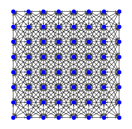
The most important is the parameter L, which by default is equal to 3. The following table shows the worst-case approximation ratio as a function of the value assigned to L.
The table also reports the number of arcs in the network flow model as a function of the number of bins n contained in the convex hull of the support points of the histograms given in input with matrix Coordinates.
| L | 1 | 2 | 3 | 5 | 10 | 15 |
Worst-case error | 7.61% | 2.68% | 1.29% | 0.49% | 0.12% | 0.06% |
Number of arcs | O(8n) | O(16n) | O(32n) | O(80n) | O(256n) | O(576n) |
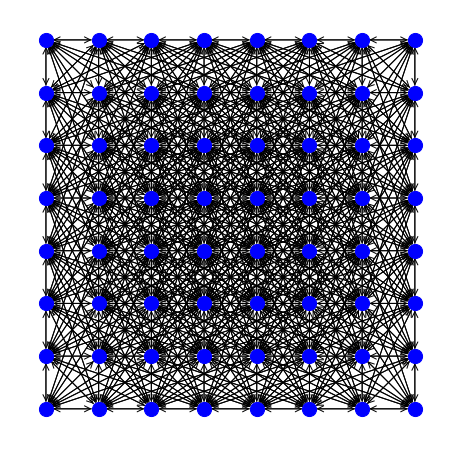
The following two figures show the network build on a grid with 8x8 nodes and using L=2 and L=3.
Value
Return an R List with the following named attributes:
distance: The value of the KW-distance between the two input histograms.status: Status of the solver used to compute the distances.runtime: Overall runtime in seconds to compute all the distances.iterations: Overall number of iterations of the Network Simplex algorithm.nodes: Number of nodes in the network model used to compute the distances.arcs: Number of arcs in the network model used to compute the distances.
See Also
See also compareOneToMany, compareAll, focusArea, Histogram2D, and Solver.
Examples
# Define a simple example
library(SpatialKWD)

# Random coordinates
N = 90
Xs <- as.integer(runif(N, 0, 31))
Ys <- as.integer(runif(N, 0, 31))
coordinates <- matrix(c(Xs, Ys), ncol=2, nrow=N)

# Random weights
test1 <- matrix(runif(2*N, 0, 1), ncol=2, nrow=N)

# Compute distance
print("Compare one-to-one with exact algorithm:")
d <- compareOneToOne(coordinates, Weights=test1, method="exact",
                     recode=TRUE, verbosity = "info")
cat("runtime:", d$runtime, " distance:", d$distance,
    " nodes:", d$nodes, " arcs:", d$arcs, "\n")

print("Compare one-to-one with approximate algorithm:")
d <- compareOneToOne(coordinates, Weights=test1, L=2, recode=TRUE)
cat("L: 2, runtime:", d$runtime, " distance:", d$distance,
    " nodes:", d$nodes, " arcs:", d$arcs, "\n")

d <- compareOneToOne(coordinates, Weights=test1, L=3)
cat("L: 3 runtime:", d$runtime, " distance:", d$distance, "\n")

d <- compareOneToOne(coordinates, Weights=test1, L=10)
cat("L: 10, runtime:", d$runtime, " distance:", d$distance, "\n")
Compute the KWD tranport distance within a given focus area
Description
This function computes the Kantorovich-Wasserstein distance within a given focus area embedded into a large region described as a grid map. Both the focus and the embedding areas are are described by spatial histograms, similarly to the input data of the other functions of this package.
The grid map is described by the two lists Xs and Ys of N coordinates, which specify the coordinates of the centroid of every single tile.
For each tile i with coordinates Xs[i], Ys[i], we have an entry in the two lists of weights W1 and W2, one for the first histograms, and the other for the second histogram.
The two lists of coordinates Xs and Ys are passed to the focusArea function as a matrix with N rows and two columns.
The two lists of weights W1 and W2 are passed as a matrix with N rows and two columns, a column for each histogram.
The focus area is specified by three parameters: the coordinates x and y of the center of the focus area, and the (circular) radius of the focus area.
The pair of coordinates (x,y) must correspond to a pair of coordinates contained in the vectors Xs,Ys.
Every tile whose distance is less or equal to the radius will be included in the focus area.
The focus area by default is circular, that is, the area is based on a L_2 norm. By setting the parameter area to the value linf it is possible to obtain
a squared focus area, induced by the norm L_infinity.
Usage
focusArea(Coordinates, Weights, x, y, radius,
           L = 3, recode = TRUE,
           method = "approx",    algorithm = "colgen",
           model="mincostflow",  verbosity = "silent",
           timelimit = 14400,    opt_tolerance = 1e-06,
           area = "l2")
Arguments
Coordinates |
A
|
Weights |
A
|
x |
Horizontal coordinate of the centroid of the focus area. |
y |
Vertical coordinate of the centroid of the focus area. |
radius |
The radius of the focus area. |
L |
Approximation parameter. Higher values of L give a more accurate solution, but they require a longer running time. Data type: positive integer. |
recode |
If equal to |
method |
Method for computing the KW distances: |
algorithm |
Algorithm for computing the KW distances: |
model |
Model for building the underlying network: |
verbosity |
Level of verbosity of the log: |
timelimit |
Time limit in second for running the solver. |
opt_tolerance |
Numerical tolerance on the negative reduced cost for the optimal solution. |
area |
Type of norm for delimiting the focus area: |
Details
The function focusArea(Coordinates, Weights, x, y, radius, ...) computes the KW distance within a focus area by implicitly considering the surrounding larger area.
The mass contained within the focus area is transported to a destination either within or outside the focus area.
All the mass contained outside the focus area could be used to balance the mass within the focus area.
Value
Return an R List with the following named attributes:
distance: The value of the KW-distance between the two input areas.status: Status of the solver used to compute the distances.runtime: Overall runtime in seconds to compute all the distances.iterations: Overall number of iterations of the Capacitated Network Simplex algorithm.nodes: Number of nodes in the network model used to compute the distances.arcs: Number of arcs in the network model used to compute the distances.
See Also
See also compareOneToOne, compareOneToMany, compareAll, Histogram2D, and Solver.
Examples
# Define a simple example
library(SpatialKWD)

# Random coordinates
N = 90
Xs <- as.integer(runif(N, 0, 31))
Ys <- as.integer(runif(N, 0, 31))
coordinates <- matrix(c(Xs, Ys), ncol=2, nrow=N)

# Random weights
test1 <- matrix(runif(2*N, 0, 1), ncol=2, nrow=N)

# Compute distance
print("Compare one-to-one with exact algorithm:")
d <- focusArea(coordinates, Weights=test1,
                x=15, y=15, radius=5,
                method="exact", recode=TRUE, verbosity = "info")
cat("runtime:", d$runtime, " distance:", d$distance,
    " nodes:", d$nodes, " arcs:", d$arcs, "\n")
Two Dimensional Histogram for Spatial Data
Description
The Histogram2D class represents a single spatial 2-dimensional histograms. The class is mainly composed of three vectors of the same length n. The first two vectors of integers, called Xs and Ys, give the coordinates of each bin of the histogram, while the third
vector of doubles, called Ws, gives the weight Ws[i] of the i-th bin located at position Xs[i] and Ys[i].
A 2D histogram can be also defined by adding (or updating) a single element a the time (see the second constructor).
Note that the positions of the bins are not required to lay on rectangular (or squared) grid, but they can lay everywhere in the plane. Before computing the distance between a pair of algorithms, the solver will compute a convex hull of all non-empty bins.
Arguments
n |
Number of non-empty bins. Type: positive integer. |
Xs |
Vector of horizontal coordinates the bins. Type: vector of integers. |
Ys |
Vector of vertical coordinates the bins. Type: vector of integers. |
Ws |
Vector of positive weights of the bin at position (x,y). Type: vector of positive doubles. |
x |
Horizontal coordinate of a bin. Type: integer. |
y |
Vertical coordinate of a bin. Type: integer. |
w |
Weight of the bin at position (x,y). Type: positive double. |
u |
Weight of the bin to be added to the weight at position (x,y). If a bin in position (x,y) is absent, then it is added with weight equal to |
Details
The public methods of the Histogram2D class are described below.
Value
The add, update, and normalize does not return any value.
The size method returns the number of non-empty bins in h.
The balance method returns the sum of the weights in h.
Methods
Histogram2D(n, Xs, Ys, Ws):c'tor.
add(x, y, w):it adds a bin located at position (x,y) with weight w.
update(x, y, u):return the total mass balance of this histogram, that is, return the quantity
\sum_{i=1,\dots,n} w_i.size():return the number of non-empty bins n of this histogram.
normalize():normalize the weights of all non-empty bins, such that they all sum up to 1. Indeed, this method implements the operation:
w_i \gets \frac{w_i}{\sum_{i=1,\dots,n} w_i}.balance():return the total mass balance of this histogram, that is, return the quantity
\sum_{i=1,\dots,n} w_i.
See Also
See also compareOneToOne, compareOneToMany, compareAll, focusArea, and Solver.
Examples
library(SpatialKWD)

# Define a simple histogram
h <- new(Histogram2D)

# Add half unit of mass at positions (1,0) and (0,1)
h$add(1, 0, 0.5)
h$add(0, 1, 0.5)

# Add at position (5,5) a unit of mass
h$add(5, 5, 1)

# Normalize the histogram
h$normalize()

# Print the total weight (mass) of the histogram
print(sprintf("Histogram total weight = %f", h$balance()))
Spatial-KWD Solver
Description
The Solver class is the main wrapper to the core algorithms implemented in the Spatial KWD package.
It has several methods that permit to compare two, or more, objects of type Histogram2D.
If you use the helper functions described at the begging of this document, you can avoid using this class directly
Arguments
n |
Number of bins in the histograms |
H1 |
First object of type |
H2 |
Second object of type |
L |
Approximation parameter. Higher values of L give a more accurate solution, but they require a longer running time. Table X gives the guarantee approximation bound as a function of L. Type: positive integer. |
Xs |
Vector of horizontal coordinates the bins. Type: vector of integers. |
Ys |
Vector of vertical coordinates the bins. Type: vector of integers. |
W1 |
Vector of weights of the bin at the positions specified by |
W2 |
Vector of weights of the bin at the positions specified by |
Ws |
Matrix of weights of the bin at the positions specified by |
name |
Name of the parameter to set and/or get. Type: string. |
value |
Value to set the corresponding parameter specified by |
Details
The public methods of this class are:
The Solver class can be controlled by the list of parameters given in the following table, which can be set with the setParam(name, value) method. A detailed description of each parameter is given below.
| Parameter Name | Possible Values | Default Value |
Method | exact, approx | approx |
Model | bipartite, mincostflow | mincostflow |
Algorithm | fullmodel, colgen | colgen |
Verbosity | silent, info, debug | info |
TimeLimit | Any positive integer smaller than INTMAX | INTMAX |
OptTolerance | Any value in [10^{-9}, 10^{-1}] | 10^{-6}
|
-
Method: set which method to use for computing the exact distance between a pair of histograms. The options for this parameter are:-
exact: Compute the exact KW distance. This method is only helpful for small and sparse spatial maps. -
approx: Compute an approximation KW distance which depends on the parameter L. This is the default value.
-
-
Model: set which network model to use for computing the exact distance between a pair of histograms. The options for this parameter are:-
bipartite: Build a complete bipartite graph. This method is only helpful for small and sparse spatial maps. -
mincostflow: Build an uncapacitated network flow. This is, in general, smaller than thebipartitemodel, except for very sparse histograms.
-
-
Algorithm: set which algorithm to use to compute an approximate distance between a pair of histograms, which depends on the parameter L. The options for this parameter are:-
fullmodel: Build a complete network model and solve the corresponding problem. -
colgen: Build the network model incrementally while computing the KW distance. It is the recommended method for very large dense spatial maps. On medium and small spatial maps, the fullmodel could be faster.
The default value is set to
colgen. -
-
Verbosity: set the level of verbosity of the logs. Possible values aresilent,info,debug. The last is more verbose than the other two. The default value is set toinfo. -
TimeLimit: set the time limit for computing the distance between a pair of spatial maps. Min values:INTMAX. The default value is set toINTMAX. -
OptTolerance: Optimality tolerance on negative reduced cost variables to enter the basis. Min value:10^{-9}, max value:10^{-1}. The default value is set to10^{-6}.
Methods
compareExact(Xs, Ys, W1, W2):compute the exact distance between the two vector of weights
W1andW2, on the convex hull of the points defined by the two vectorsXsandYs. The algorithm used by the solver is controlled by the parameterExactMethod(see below). This method returns a single value (double), which is the KW-distance betweenW1andW2.compareExact(Xs, Ys, W1, Ws):compute the exact distances between the vector of weights
W1and each of the vector of weights inWs, on the convex hull of the points defined by the two vectorsXsandYs. The algorithm used by the solver is controlled by the parameterExactMethod(see below). This method returns a vector of double of the same size ofWs, representing the distance ofW1to every element ofWs.compareExact(Xs, Ys, Ws):compute a symmetric matrix of pairwise exact distances between all the possible pairs of the vector listed in
Ws. The algorithm used by the solver is controlled by the parameterExactMethod(see below).compareApprox(Xs, Ys, W1, W2, L):compute the approximate distance between the two vector of weights
W1andW2, on the convex hull of the points defined by the two vectorsXsandYs. The parameterApproxMethod(see below) controls the algorithm used by the solver. This method returns a single value (double), which is the KW-distance betweenW1andW2.compareApprox(Xs, Ys, W1, Ws, L):compute the approximate distances between the vector of weights
W1and each of the vector of weights inWs, on the convex hull of the points defined by the two vectorsXsandYs. The parameterApproxMethod(see below) controls the algorithm used by the solver. This method returns a vector of double of the same size ofWs, representing the distance ofW1to every element ofWs.compareApprox(Xs, Ys, Ws, L):compute a symmetric matrix of pairwise approximate distances (which depends on the value of L) between all the possible pairs of the vector listed in
Ws. The parameterApproxMethod(see below) controls the algorithm used by the solver.runtime():return the runtime in seconds to the last call to one of the compare methods. It reports the runtime of the execution of the Network Simplex algorithm.
preprocesstime():return the preprocessing time in seconds to the last call to one of the compare methods. It reports the execution time to set up the main data structures and to compute the convex hull of all the input histograms.
setParam(name, value):set the parameter
nameto the newvalue. Every parameter has a default value. See below for the existing parameters.getParam(name):return the current value of the parameter
name.
See Also
See also compareOneToOne, compareOneToMany, compareAll, focusArea, and Histogram2D.