| Type: | Package |
| Title: | Agricultural Datasets |
| Version: | 1.26 |
| Description: | Datasets from books, papers, and websites related to agriculture. Example graphics and analyses are included. Data come from small-plot trials, multi-environment trials, uniformity trials, yield monitors, and more. |
| License: | MIT + file LICENSE |
| URL: | https://kwstat.github.io/agridat/ |
| BugReports: | https://github.com/kwstat/agridat/issues |
| Suggests: | AER, agricolae, betareg, broom, car, coin, corrgram, desplot, dplyr, effects, emmeans, equivalence, FrF2, gam, gge, ggplot2, gnm, gstat, HH, knitr, lattice, latticeExtra, lme4, lucid, mapproj, maps, MASS, MCMCglmm, metafor, mgcv, nlme, nullabor, ordinal, pbkrtest, pls, pscl, qicharts, qtl, reshape2, rmarkdown, sp, SpATS, survival, testthat, vcd |
| VignetteBuilder: | knitr |
| Encoding: | UTF-8 |
| Language: | en-US |
| LazyData: | true |
| RoxygenNote: | 7.3.3 |
| NeedsCompilation: | no |
| Packaged: | 2025-11-14 21:44:23 UTC; wrightkevi |
| Author: | Kevin Wright  [aut, cre, cph]
 |
| Maintainer: | Kevin Wright <kw.stat@gmail.com> |
| Repository: | CRAN |
| Date/Publication: | 2025-11-19 06:10:48 UTC |
Datasets from agricultural experiments
Description
This package contains datasets from publications relating to agriculture, including field crops, tree crops, animal studies, and a few others.
Details
If you use these data, please cite both the agridat package and the original source of the data.
Abbreviations in the 'other' column include: xy = coordinates, pls = partial least squares, rsm = response surface methodology, row-col = row-column design, ts = time series,
Uniformity trials with a single genotype
Yield monitor
| name | reps | years | trt | other | model |
| gartner.corn | xy,ym | ||||
| lasrosas.corn | 3 | 2 | 6 | xy,ym | lm |
| kayad.alfalfa | 4 | xy,ym |
Animals
| name | gen | years | trt | other | model |
| alwan.lamb | 34 | 2 | ordinal | clmm | |
| becker.chicken | 5,12 | heritability | lmer | ||
| crampton.pig | 5 | 2 cov | lm | ||
| brandt.switchback | 10 | 2 | aov | ||
| depalluel.sheep | 4 | 4 | latin | ||
| diggle.cow | 4 | ts | |||
| foulley.calving | ordinal | polr | |||
| goulden.eggs | controlchart | ||||
| harvey.lsmeans | 3,3 | lm | |||
| harville.lamb | 5 | lmer | |||
| henderson.milkfat | nls,lm,glm,gam | ||||
| holland.arthropods | 5 | ||||
| ilri.sheep | 4 | 6 | diallel | lmer, asreml | |
| kenward.cattle | 2 | asreml | |||
| lucas.switchback | 12 | 3 | aov | ||
| mead.lamb | 3 | 3 | glm | ||
| patterson.switchback | 12 | 4 | aov | ||
| urquhart.feedlot | 11 | 3 | lm | ||
| woodman.pig | 3 | cov | lm | ||
| zuidhof.broiler | ts |
Trees
| name | gen | loc | reps | years | trt | other | model |
| box.cork | repeated | radial, asreml | |||||
| devries.pine | 4 | 3,3 | xy,graeco | aov | |||
| harris.wateruse | 2 | 2 | repeated | asreml,lme | |||
| hanover.whitepine | 7*4 | 4 | heritability | lmer | |||
| johnson.douglasfir | xy | ||||||
| lavoranti.eucalyptus | 70 | 7 | svd | ||||
| pearce.apple | 4 | 6 | cov | lm,lmer | |||
| williams.trees | 37 | 6 | 2 |
Field and horticulture crops
| name | gen | loc | reps | years | trt | other | model |
| acorsi.grayleafspot | 36 | 9 | 2 | 5 | nonnormal | gnm,ammi | |
| adugna.sorghum | 28 | 13 | 5 | ||||
| aastveit.barley | 15 | 9 | yr*gen~yr*trt | pls | |||
| allcroft.lodging | 32 | 7 | percent | tobit | |||
| archbold.apple | 2 | 5 | 24 | split-split | lmer | ||
| ars.earlywhitecorn96 | 60 | 9 | 6 traits | dotplot | |||
| australia.soybean | 58 | 4 | 2 | 4-way, 6 traits | biplot | ||
| bachmaier.nitrogen | 4 | 2,11 | quadratic lm | ||||
| barrero.maize | 847 | 16 | 4 | 11 | 6 | gain,asreml | |
| battese.survey | 12 | 1-5 | 2 | lmer | |||
| beall.webworms | 15 | 2,2 | xy, split-block | glm poisson,nb | |||
| beaven.barley | 8 | 20 | xy | ||||
| belamkar.augmented | 273 | 8 | xy, incblock | asreml | |||
| besag.bayesian | 75 | 3 | xy | asreml | |||
| besag.beans | 6 | 4*6 | xy | lm,competition | |||
| besag.checks | 2 | xy | |||||
| besag.elbatan | 50 | 3 | xy | lm, gam | |||
| besag.endive | xy,binary | autologistic | |||||
| besag.met | 64 | 6 | 3 | xy, incblock | asreml, lme | ||
| besag.triticale | 3 | 2,2,3 | xy | lm, asreml | |||
| bliss.borers | 4 | glm | |||||
| blackman.wheat | 12 | 7 | 2 | biplot | |||
| bond.diallel | 6*6 | 9 | diallel | ||||
| bridges.cucumber | 4 | 2 | 4 | xy, latin, hetero | asreml | ||
| brandle.rape | 5 | 9 | 3 | lmer | |||
| buntaran.wheat | 30 | 18 | 2 | alpha | asreml | ||
| burgueno.alpha | 15 | 3 | xy, alpha | asreml,lmer | |||
| burgueno.rowcol | 64 | 2 | xy, row-col | asreml,lmer | |||
| burgueno.unreplicated | 280 | xy | asreml | ||||
| butron.maize | 49 | 3 | 2 | diallel,pedigree | biplot,asreml | ||
| caribbean.maize | 17 | 4 | 3 | ||||
| carmer.density | 8 | 4 | nls,nlme | ||||
| carlson.germination | 15 | 8 | glm | ||||
| chakravertti.factorial | 3 | 3 | 3,5,3,3 | factorial | aov | ||
| chinloy.fractionalfactorial | 9 | 1/3 3^5 = 3,3,3,3 | xy,factorial | aov | |||
| christidis.competition | 9 | 5 | xy | ||||
| cochran.beets | 6 | 7 | |||||
| cochran.bib | 13 | 13 | bib | aov, lme | |||
| cochran.crd | 7 | xy, crd | aov | ||||
| cochran.factorial | 2 | 2,2,2,2 = 2^4 | factorial | aov | |||
| cochran.latin | 6 | 6 | xy, latin | aov | |||
| cochran.lattice | 5 | 16 | xy, latin | lmer | |||
| cochran.wireworms | 5 | 5 | xy, latin | glm | |||
| cochran.eelworms | 4 | 5 | xy | aov | |||
| connolly.potato | 20 | 4 | xy, competition | lm | |||
| cornelius.maize | 9 | 20 | svd | ||||
| corsten.interaction | 20 | 7 | |||||
| cramer.cucumber | 8 | pathcoef | |||||
| crossa.wheat | 18 | 25 | ammi | ||||
| crowder.seeds | 2 | 21 | 2 | glm,INLA,jags | |||
| cox.stripsplit | 4 | 3,4,2 | split-block | aov | |||
| cullis.earlygen | 532 | xy | asreml | ||||
| damesa.maize | 22 | 4 | 3 | xy,incblock,twostage | asreml | ||
| dasilva.maize | 55 | 9 | 3 | ||||
| darwin.maize | 12 | 2 | t.test | ||||
| davidian.soybean | 2 | 3 | nlme | ||||
| denis.missing | 5 | 26 | lme | ||||
| denis.ryegrass | 21 | 7 | aov | ||||
| digby.jointregression | 10 | 17 | 4 | lm | |||
| durban.competition | 36 | 3 | xy, competition | lm | |||
| durban.rowcol | 272 | 2 | xy | lm, gam, asreml | |||
| durban.splitplot | 70 | 4 | 2 | xy | lm, gam, asreml | ||
| eden.potato | 4 | 3 | 4-12 | xy, rcb, latin | aov | ||
| eden.nonnormal | 4 | 4 | aov | ||||
| edwards.oats | 80 | 5 | 3 | 7 | |||
| engelstad.nitro | 2 | 5 | 6 | rsm1 | nls quadratic plateau | ||
| fan.stability | 13 | 10 | 2 | 3-way | stability | ||
| federer.diagcheck | 122 | xy | lm, lmer, asreml | ||||
| federer.tobacco | 8 | 7 | xy | lm | |||
| fisher.barley | 5 | 6 | 2 | ||||
| fisher.latin | 5 | 5 | xy,latin | lm | |||
| fox.wheat | 22 | 14 | lm | ||||
| gathmann.bt | 2 | 8 | tost | ||||
| gauch.soy | 7 | 7 | 4 | 12 | ammi | ||
| george.wheat | 211 | 9 | 4 | 15 | |||
| giles.wheat | 19 | 13 | 2 traits | gnm | |||
| gilmour.serpentine | 108 | 3 | xy, serpentine | asreml | |||
| gilmour.slatehall | 25 | 6 | xy | asreml | |||
| gomez.fractionalfactorial | 2 | 1/2 2^6 = 2,2,2,2,2,2 | xy,factorial | lm | |||
| gomez.groupsplit | 45 | 3 | 2 | xy, 3 gen groups | aov | ||
| gomez.heteroskedastic | 35 | 3 | hetero | ||||
| gomez.multilocsplitplot | 2 | 3 | 3 | rsm1,nitro | aov, lmer | ||
| gomez.nitrogen | 4 | 8 | aov, contrasts | ||||
| gomez.nonnormal1 | 4 | 9 | log10 | lm | |||
| gomez.nonnormal2 | 14 | 3 | sqrt | lm | |||
| gomez.nonnormal3 | 12 | 3 | arcsin | lm | |||
| gomez.seedrate | 4 | 6 | rate | lm | |||
| gomez.splitplot.subsample | 3 | 8,4 | subsample | aov | |||
| gomez.splitsplit | 3 | 3 | xy, nitro, mgmt | aov, lmer | |||
| gomez.stripplot | 6 | 3 | xy, nitro | aov | |||
| gomez.stripsplitplot | 6 | 3 | xy, nitro | aov | |||
| gomez.wetdry | 3 | 2 | 5 | nitro | lmer | ||
| gotway.hessianfly | 16 | 4 | xy | lmer | |||
| goulden.latin | 5 | 5 | xy, latin | lm | |||
| goulden.splitsplit | 2 | 4 | 2*5 | xy, split | aov | ||
| graybill.heteroskedastic | 4 | 13 | hetero | ||||
| gregory.cotton | 2 | 4*3*2*2 | polar | ||||
| grover.diallel | 4 | 6*6 | diallel | lmDiallel | |||
| grover.rcb.subsample | 4 | 2 | 9 | subsample | aov | ||
| gumpertz.pepper | xy | glm | |||||
| hadasch.lettuce | 89 | 3 | 3 | markers | asreml | ||
| hanks.sprinkler | 3 | 3 | xy | asreml | |||
| hayman.tobacco | 8 | 2 | 2 | diallel | asreml | ||
| hazell.vegetables | 4 | 6 | linprog | ||||
| heady.fertilizer | 2 | 9*9 | rsm2 | lm,rgl | |||
| hernandez.nitrogen | 5 | 4 | rsm1 | lm, nls | |||
| hildebrand.systems | 14 | 4 | asreml | ||||
| holshouser.splitstrip | 4 | 4 | 2*4 | rsm1,pop | lmer | ||
| huehn.wheat | 20 | 10 | huehn | ||||
| hughes.grapes | 3 | 6 | binomial | lmer, aod, glmm | |||
| hunter.corn | 12 | 3 | 1 | rsm1 | xyplot | ||
| ivins.herbs | 13 | 6 | 2 traits | lm, friedman | |||
| jansen.apple | 3 | 4 | 3 | binomial | glmer | ||
| jansen.carrot | 16 | 3 | 2 | binomial | glmer | ||
| jansen.strawberry | 12 | 4 | ordinal | mosaicplot | |||
| jayaraman.bamboo | 6 | 2 | 3 | heritability | lmer | ||
| jenkyn.mildew | 9 | 4 | lm | ||||
| john.alpha | 24 | 3 | xy, alpha | lm, lmer | |||
| johnson.blight | 2 | logistic | |||||
| kang.maize | 17 | 4 | 3 | 2,4 | |||
| kang.peanut | 10 | 15 | 4 | gge | |||
| karcher.turfgrass | 4 | 2,4 | ordinal | polr | |||
| keen.potatodamage | 6 | 4 | 2,3,8 | ordinal | mosaicplot,clmm | ||
| kempton.competition | 36 | 3 | xy, competition | lme AR1 | |||
| kempton.rowcol | 35 | 2 | xy, row-col | lmer | |||
| kling.augmented | 53 | 6 | xy, augmented | lmer | |||
| kempton.slatehall | 25 | 6 | xy | asreml, lmer | |||
| kirk.potato | 21 | 15 | xy | ||||
| lee.potatoblight | 337 | 4 | 11 | xy, ordinal, repeated | |||
| lehner.soybeanmold | 35 | 4 | 11 | metafor, lmer | |||
| lillemo.wheat | 24 | 13 | 7 | medpolish, huehn | |||
| lin.superiority | 33 | 12 | superiority | ||||
| lin.unbalanced | 33 | 18 | superiority | ||||
| linder.wheat | 9 | 7 | 4 | gge | |||
| little.splitblock | 4 | 4,5 | xy, split-block | aov | |||
| lonnquist.maize | 11 | diallel | asreml | ||||
| lyons.wheat | 12 | 4 | |||||
| lu.stability | 5 | 6 | huehn | ||||
| mcconway.turnip | 2 | 4 | 2,4 | hetero | aov, lme | ||
| mcleod.barley | 8 | 6 | aggregate | ||||
| mead.cauliflower | 2 | poisson | glm | ||||
| mead.cowpea.maize | 3,2 | 3 | 4 | intercrop | |||
| mead.germination | 4 | 4,4 | binomial | glm | |||
| mead.strawberry | 8 | 4 | |||||
| mead.turnip | 3 | 5,4 | aov | ||||
| miguez.biomass | 3 | 4 | |||||
| minnesota.barley.weather | 6 | 10 | |||||
| minnesota.barley.yield | 22 | 6 | 10 | dotplot | |||
| omer.sorghum | 18 | 6 | 4 | jags | |||
| onofri.winterwheat | 8 | 3 | 7 | ammi | |||
| ortiz.tomato | 15 | 18 | 16 | env*gen~env*cov | pls | ||
| pacheco.soybean | 18 | 11 | ammi | ||||
| payne.wheat | 20 | 6 | rotation | asreml | |||
| pederson.lettuce.repeated | 18 | 3 | nlme | ||||
| perry.springwheat | 28 | 5 | 4 | gain | lm,lmer,asreml | ||
| petersen.sorghum.cowpea | 2 | 4 | 7 | 4 | intercrop | ||
| piepho.cocksfoot | 25 | 7 | mumm | ||||
| ratkowsky.onions | lm | ||||||
| reid.grasses | 4 | 3 | 21 | nlme SSfpl | |||
| riddle.wheat | 25 | 5 | 2 | xy, latin | aov | ||
| ridout.appleshoots | 30 | 2,4 | zip | zeroinfl | |||
| rothamsted.brussels | 4 | 6 | |||||
| rothamsted.oats | 8 | 9 | rcb | ||||
| ryder.groundnut | 5 | 4 | xy, rcb | lm | |||
| salmon.bunt | 10 | 2 | 20 | betareg | |||
| senshu.rice | 40 | lm,Fieller | |||||
| shafii.rapeseed | 6 | 14 | 3 | 3 | biplot | ||
| shaw.oats | 13 | 2 | 5 | 3 | aov | ||
| sharma.met | 7 | 3 | 3 | 2 | FinlayWilkinson | ||
| silva.cotton | 5 | 5 | 5 traits | glm,poisson | |||
| sinclair.clover | 5,5 | rsm2,mitzerlich | nls,rgl | ||||
| snedecor.asparagus | 4 | 4 | 4 | split-plot, antedependence | |||
| snijders.fusarium | 17 | 3 | 4 | percent | glm/gnm,gammi | ||
| steptoe.morex.pheno | 152 | 16 | 10 traits | ||||
| steptoe.morex.geno | 150 | 223 markers, qtl | |||||
| streibig.competition | 2 | 3 | glm | ||||
| stroup.nin | 56 | 4 | xy | asreml | |||
| stroup.splitplot | 4 | asreml, MCMCglmm | |||||
| student.barley | 2 | 51 | 6 | lmer | |||
| tai.potato | 8 | 3 | 2 | tai | |||
| talbot.potato | 9 | 12 | gen*env~gen*trt | pls | |||
| tesfaye.millet | 47 | 2 | 2-3 | 2 | 4 | xy | asreml |
| theobald.barley | 3 | 5 | 2 | 5 | rsm1 | ||
| theobald.covariate | 10 | 7 | 5 | cov | jags | ||
| thompson.cornsoy | 5 | 33 | repeated measures | aov | |||
| vaneeuwijk.fusarium | 20 | 4 | 7 | 3-way | aov | ||
| vaneeuwijk.drymatter | 6 | 4 | 7 | 3-way | aov,lmer | ||
| vaneeuwijk.nematodes | 11 | nonnormal,poisson | gnm, gammi | ||||
| vargas.wheat1 | 7 | 6 | gen*yr~gen*trt, yr*gen~yr*cov | pls | |||
| vargas.wheat2 | 8 | 7 | env*gen~env*cov | pls | |||
| vargas.txe | 10 | 24 | yr*trt~yr*cov | pls | |||
| verbyla.lupin | 9 | 8 | 3 | 2 | 7 | rsm1, xy, density | asreml |
| vold.longterm | 19 | 4 | rsm1 | nls,nlme | |||
| vsn.lupin3 | 336 | 3 | xy | asreml | |||
| wedderburn.barley | 10 | 9 | percent | glm/gnm | |||
| weiss.incblock | 31 | 6 | xy,incblock | asreml | |||
| weiss.lattice | 49 | 4 | xy,lattice | lm,asreml | |||
| welch.bermudagrass | 4,4,4 | rsm3, factorial | lm, jags | ||||
| wheatley.carrot | 3 | 11 | glm-binomial | ||||
| yan.winterwheat | 18 | 9 | gge,biplot | ||||
| yang.barley | 6 | 18 | biplot | ||||
| yates.missing | 10 | 3^2 = 3,3 | factorial | lm, pca | |||
| yates.oats | 3 | 6 | xy,split,nitro | lmer |
Time series
| name | years | trt | other | model |
| byers.apple | lme | |||
| broadbalk.wheat | 74 | 17 | ||
| hessling.argentina | 30 | temp,precip | ||
| kreusler.maize | 4 | 5 | plant growth | |
| lambert.soiltemp | 1 | 7 | ||
| nass.barley | 146 | |||
| nass.corn | 146 | |||
| nass.cotton | 146 | |||
| nass.hay | 104 | |||
| nass.sorghum | 93 | |||
| nass.wheat | 146 | |||
| nass.rice | 117 | |||
| nass.soybean | 88 | |||
| usda.gmoadoption | 31 | 5 | ||
| walsh.cottonprice | 34 | cor |
Other
| name | model |
| cate.potassium | cate-nelson |
| cleveland.soil | loess 2D |
| harrison.priors | nls, prior |
| nebraska.farmincome | choropleth |
| pearl.kernels | chisq |
| stirret.borers | lm, 4 trt |
| turner.herbicide | glm, 4 trt |
| usgs.herbicides | non-detect |
| wallace.iowaland | lm, choropleth |
| waynick.soil | spatial, nitro/carbon |
Summaries:
Diallel experiments:
| name | gen | loc | reps | trt | model |
| bond.diallel | 6*6 | 9 | |||
| butron.maize | 49 | 3 | biplot,asreml | ||
| grover.diallel | 4 | 6*6 | lmDiallel | ||
| hayman.tobacco | 8 | 2 | asreml | ||
| ilri.sheep | 4 | 6 | |||
| lonnquist.maize | 11 | asreml |
Factorial experiments:
| name | gen | loc | reps | years | trt | other | model |
| chakravertti.factorial | 3 | 3 | 3,5,3,3 | factorial | aov | ||
| chinloy.fractionalfactorial | 9 | 1/3 3^5 = 3,3,3,3 | xy,factorial | aov | |||
| cochran.factorial | 2 | 2,2,2,2 = 2^4 | factorial | aov | |||
| gomez.fractionalfactorial | 2 | 1/2 2^6 = 2,2,2,2,2,2 | xy,factorial | lm | |||
| welch.bermudagrass | 4,4,4 | rsm3, factorial | lm, jags | ||||
| yates.missing | 10 | 3^2 = 3,3 | factorial | lm, pca |
Multi-environment trials with multi-genotype,loc,rep,year:
| name | gen | loc | reps | years | trt | other | model |
| barrero.maize | 847 | 16 | 4 | 11 | 6 | asreml | |
| edwards.oats | 80 | 5 | 3 | 7 | |||
| gauch.soy | 7 | 7 | 4 | 12 | ammi | ||
| george.wheat | 211 | 9 | 4 | 15 | |||
| shafii.rapeseed | 6 | 14 | 3 | 3 | biplot | ||
| shaw.oats | 13 | 2 | 5 | 3 | aov | ||
| tesfaye.millet | 47 | 2 | 2-3 | 2 | 4 | xy,FA | asreml |
| verbyla.lupin | 9 | 8 | 3 | 2 | 7 | rsm1, xy, density | asreml |
Data with markers: hadasch.lettuce.markers, steptoe.morex.geno
Data with pedigree: butron.maize
Author(s)
Kevin Wright, with support from many people who granted permission to include their data in this package.
References
J. White and Frits van Evert. (2008). Publishing Agronomic Data. Agron J. 100, 1396-1400. https://doi.org/10.2134/agronj2008.0080F
Barley heights and environmental covariates in Norway
Description
Average height for 15 genotypes of barley in each of 9 years. Also 19 covariates in each of the 9 years.
Usage
data("aastveit.barley.covs")
data("aastveit.barley.height")
Format
The 'aastveit.barley.covs' dataframe has 9 observations on the following 20 variables.
yearyear
R1avg rainfall (mm/day) in period 1
R2avg rainfall (mm/day) in period 2
R3avg rainfall (mm/day) in period 3
R4avg rainfall (mm/day) in period 4
R5avg rainfall (mm/day) in period 5
R6avg rainfall (mm/day) in period 6
S1daily solar radiation (ca/cm^2) in period 1
S2daily solar radiation (ca/cm^2) in period 2
S3daily solar radiation (ca/cm^2) in period 3
S4daily solar radiation (ca/cm^2) in period 4
S5daily solar radiation (ca/cm^2) in period 5
S6daily solar radiation (ca/cm^2) in period 6
STsowing time, measured in days after April 1
T1avg temp (deg Celsius) in period 1
T2avg temp (deg Celsius) in period 2
T3avg temp (deg Celsius) in period 3
T4avg temp (deg Celsius) in period 4
T5avg temp (deg Celsius) in period 5
T6avg temp (deg Celsius) in period 6
The 'aastveit.barley.height' dataframe has 135 observations on the following 3 variables.
yearyear, 9 years spanning from 1974 to 1982
gengenotype, 15 levels
heightheight (cm)
Details
Experiments were conducted at As, Norway.
The height dataframe contains average plant height (cm) of 15 varieties
of barley in each of 9 years.
The growth season of each year was divided into eight periods from sowing to harvest. Because the plant stop growing about 20 days after ear emergence, only the first 6 periods are included here.
Used with permission of Harald Martens.
Source
Aastveit, A. H. and Martens, H. (1986). ANOVA interactions interpreted by partial least squares regression. Biometrics, 42, 829–844. https://doi.org/10.2307/2530697
References
J. Chadoeuf and J. B. Denis (1991). Asymptotic variances for the multiplicative interaction model. J. App. Stat., 18, 331-353. https://doi.org/10.1080/02664769100000032
Examples
## Not run:

library(agridat)
data("aastveit.barley.covs")
data("aastveit.barley.height")

libs(reshape2, pls)

  # First, PCA of each matrix separately

  Z <- acast(aastveit.barley.height, year ~ gen, value.var="height")
  Z <- sweep(Z, 1, rowMeans(Z))
  Z <- sweep(Z, 2, colMeans(Z)) # Double-centered
  sum(Z^2)*4 # Total SS = 10165
  sv <- svd(Z)$d
  round(100 * sv^2/sum(sv^2),1) # Prop of variance each axis
  # Aastveit Figure 1.  PCA of height
  biplot(prcomp(Z),
         main="aastveit.barley - height", cex=0.5)

  U <- aastveit.barley.covs
  rownames(U) <- U$year
  U$year <- NULL
  U <- scale(U) # Standardized covariates
  sv <- svd(U)$d
  # Proportion of variance on each axis
  round(100 * sv^2/sum(sv^2),1)

  # Now, PLS relating the two matrices
  m1 <- plsr(Z~U)
  loadings(m1)
  # Aastveit Fig 2a (genotypes), but rotated differently
  biplot(m1, which="y", var.axes=TRUE)
  # Fig 2b, 2c (not rotated)
  biplot(m1, which="x", var.axes=TRUE)

  # Adapted from section 7.4 of Turner & Firth,
  # "Generalized nonlinear models in R: An overview of the gnm package"
  # who in turn reproduce the analysis of Chadoeuf & Denis (1991),
  # "Asymptotic variances for the multiplicative interaction model"

  libs(gnm)
  dath <- aastveit.barley.height
  dath$year = factor(dath$year)

  set.seed(42)
  m2 <- gnm(height ~ year + gen + Mult(year, gen), data = dath)
  # Turner: "To obtain parameterization of equation 1, in which sig_k is the
  # singular value for component k, the row and column scores must be constrained
  # so that the scores sum to zero and the squared scores sum to one.
  # These contrasts can be obtained using getContrasts"
  gamma <- getContrasts(m2, pickCoef(m2, "[.]y"),
                        ref = "mean", scaleWeights = "unit")
  delta <- getContrasts(m2, pickCoef(m2, "[.]g"),
                        ref = "mean", scaleWeights = "unit")
  # estimate & std err
  gamma <- gamma$qvframe
  delta <- delta$qvframe
  # change sign of estimate
  gamma[,1] <- -1 * gamma[,1]
  delta[,1] <- -1 * delta[,1]
  # conf limits based on asymptotic normality, Chadoeuf table 8, p. 350,
  round(cbind(gamma[,1], gamma[, 1] +
                           outer(gamma[, 2], c(-1.96, 1.96))) ,3)
  round(cbind(delta[,1], delta[, 1] +
                           outer(delta[, 2], c(-1.96, 1.96))) ,3)

## End(Not run)
Multi-environment trial evaluating 36 maize genotypes in 9 locations
Description
Multi-environment trial evaluating 36 maize genotypes in 9 locations
Usage
data("acorsi.grayleafspot")Format
A data frame with 324 observations on the following 3 variables.
gengenotype, 36 levels
envenvironment, 9 levels
repreplicate, 2 levels
ygrey leaf spot severity
Details
Experiments conducted in 9 environments in Brazil in 2010-11. Each location had an RCB with 2 reps.
The response variable is the percentage of leaf area affected by gray leaf spot within each experimental unit (plot).
Acorsi et al. use this data to illustrate the fitting of a generalized AMMI model with non-normal data.
Source
C. R. L. Acorsi, T. A. Guedes, M. M. D. Coan, R. J. B. Pinto, C. A. Scapim, C. A. P. Pacheco, P. E. O. Guimaraes, C. R. Casela. (2016). Applying the generalized additive main effects and multiplicative interaction model to analysis of maize genotypes resistant to grey leaf spot. Journal of Agricultural Science. https://doi.org/10.1017/S0021859616001015
Electronic data and R code kindly provided by Marlon Coan.
References
None
Examples
## Not run:

  library(agridat)
  data(acorsi.grayleafspot)
  dat <- acorsi.grayleafspot

  # Acorsi figure 2. Note: Acorsi used cell means
  op <- par(mfrow=c(2,1), mar=c(5,4,3,2))
  libs(lattice)
  boxplot(y ~ env, dat, las=2,
          xlab="environment", ylab="GLS severity")
  title("acorsi.grayleafspot")
  boxplot(y ~ gen, dat, las=2,
          xlab="genotype", ylab="GLS severity")
  par(op)

  # GLM models

  # glm main-effects model with logit u(1-u) and wedderburn u^2(1-u)^2
  # variance functions
  # glm1 <- glm(y~ env/rep + gen + env, data=dat, family=quasibinomial)
  # glm2 <- glm(y~ env/rep + gen + env, data=dat, family=wedderburn)
  # plot(glm2, which=1); plot(glm2, which=2)

  # GAMMI models of Acorsi. See also section 7.4 of Turner
  # "Generalized nonlinear models in R: An overview of the gnm package"

  # full gnm model with wedderburn, seems to work
  libs(gnm)
  set.seed(1)
  gnm1 <- gnm(y ~  env/rep + env + gen + instances(Mult(env,gen),2),
              data=dat,
              family=wedderburn, iterMax =800)
  deviance(gnm1) # 433.8548
  # summary(gnm1)
  # anova(gnm1, test ="F")  # anodev, Acorsi table 4
  ##                          Df Deviance Resid. Df Resid. Dev       F    Pr(>F)
  ## NULL                                       647     3355.5
  ## env                       8  1045.09       639     2310.4 68.4696 < 2.2e-16 ***
  ## env:rep                   9    12.33       630     2298.1  0.7183    0.6923
  ## gen                      35  1176.23       595     1121.9 17.6142 < 2.2e-16 ***
  ## Mult(env, gen, inst = 1) 42   375.94       553      745.9  4.6915 < 2.2e-16 ***
  ## Mult(env, gen, inst = 2) 40   312.06       513      433.9  4.0889 3.712e-14 ***


  # maybe better, start simple and build up the model
  gnm2a <- gnm(y ~  env/rep + env + gen,
               data=dat,
               family=wedderburn, iterMax =800)

  # add first interaction term
  res2a <- residSVD(gnm2a, env, gen, 2)
  gnm2b <- update(gnm2a, . ~ . + Mult(env,gen,inst=1),
                  start = c(coef(gnm2a), res2a[, 1]))
  deviance(gnm2b) # 692.19

  # add second interaction term
  res2b <- residSVD(gnm2b, env, gen, 2)
  gnm2c <- update(gnm2b, . ~ . + Mult(env,gen,inst=1) + Mult(env,gen,inst=2),
                  start = c(coef(gnm2a), res2a[, 1], res2b[,1]))
  deviance(gnm2c) # 433.8548
  # anova(gnm2c) # weird error message

  # note, to build the ammi biplot, use the first column of res2a to get
  # axis 1, and the FIRST column of res2b to get axis 2. Slightly confusing
  emat <- cbind(res2a[1:9, 1], res2b[1:9, 1])
  rownames(emat) <- gsub("fac1.", "", rownames(emat))

  gmat <- cbind(res2a[10:45, 1], res2b[10:45, 1])
  rownames(gmat) <- gsub("fac2.", "", rownames(gmat))

  # match Acorsi figure 4
  biplot(gmat, emat, xlim=c(-2.2, 2.2), ylim=c(-2.2, 2.2), expand=2, cex=0.5,
         xlab="Axis 1", ylab="Axis 2",
         main="acorsi.grayleafspot - GAMMI biplot")

## End(Not run)
Multi-environment trial of sorghum at 3 locations across 5 years
Description
Multi-environment trial of sorghum at 3 locations across 5 years
Format
A data frame with 289 observations on the following 6 variables.
gengenotype, 28 levels
trialtrial, 2 levels
envenvironment, 13 levels
yieldyield kg/ha
yearyear, 2001-2005
loclocation, 3 levels
Details
Sorghum yields at 3 locations across 5 years. The trials were carried out at three locations in dry, hot lowlands of Ethiopia:
Melkassa (39 deg 21 min E, 8 deg 24 min N)
Mieso (39 deg 22 min E, 8 deg 41 min N)
Kobo (39 deg 37 min E, 12 deg 09 min N)
Trial 1 was 14 hybrids and one open-pollinated variety.
Trial 2 was 12 experimental lines.
Used with permission of Asfaw Adugna.
Source
Asfaw Adugna (2008). Assessment of yield stability in sorghum using univariate and multivariate statistical approaches. Hereditas, 145, 28–37. https://doi.org/10.1111/j.0018-0661.2008.2023.x
Examples
## Not run:

library(agridat)
data(adugna.sorghum)
dat <- adugna.sorghum

libs(lattice)
redblue <- colorRampPalette(c("firebrick", "lightgray", "#375997"))
levelplot(yield ~ env*gen, data=dat, main="adugna.sorghum gxe heatmap",
          col.regions=redblue)

# Genotype means match Adugna
tapply(dat$yield, dat$gen, mean)

# CV for each genotype.  G1..G15 match, except for G2.
# The table in Adugna scrambles the means for G16..G28
libs(reshape2)
mat <- acast(dat, gen~env,  value.var='yield')
round(sqrt(apply(mat, 1, var, na.rm=TRUE)) / apply(mat, 1, mean, na.rm=TRUE) * 100,2)

# Shukla stability.  G1..G15 match Adugna.  Can't match G16..G28.
dat1 <- droplevels(subset(dat, trial=="T1"))
mat1 <- acast(dat1, gen~env,  value.var='yield')
w <- mat1; k=15; n=8  # k=p gen, n=q env
w <- sweep(w, 1, rowMeans(mat1, na.rm=TRUE))
w <- sweep(w, 2, colMeans(mat1, na.rm=TRUE))
w <- w + mean(mat1, na.rm=TRUE)
w <- rowSums(w^2, na.rm=TRUE)
sig2 <- k*w/((k-2)*(n-1)) - sum(w)/((k-1)*(k-2)*(n-1))
round(sig2/10000,1) # Genotypes in T1 are divided by 10000

## End(Not run)
Multi-environment trial of cereal with lodging data
Description
Percent lodging is given for 32 genotypes at 7 environments.
Format
A data frame with 224 observations on the following 3 variables.
envenvironment, 1-7
gengenotype, 1-32
ypercent lodged
Details
This data is for the first year of a three-year study.
Used with permission of Chris Glasbey.
Source
D. J. Allcroft and C. A. Glasbey, 2003. Analysis of crop lodging using a latent variable model. Journal of Agricultural Science, 140, 383–393. https://doi.org/10.1017/S0021859603003332
Examples
## Not run:

library(agridat)
data(allcroft.lodging)
dat <- allcroft.lodging

# Transformation
dat$sy <- sqrt(dat$y)
# Variety 4 has no lodging anywhere, so add a small amount
dat[dat$env=='E5' & dat$gen=='G04',]$sy <- .01

libs(lattice)
dotplot(env~y|gen, dat, as.table=TRUE,
        xlab="Percent lodged (by genotype)", ylab="Variety",
        main="allcroft.lodging")

# Tobit model
libs(AER)
m3 <- tobit(sy ~ 1 + gen + env, left=0, right=100, data=dat)

# Table 2 trial/variety means
preds <- expand.grid(gen=levels(dat$gen), env=levels(dat$env))
preds$pred <- predict(m3, newdata=preds)
round(tapply(preds$pred, preds$gen, mean),2)
round(tapply(preds$pred, preds$env, mean),2)


## End(Not run)
For the 34 sheep sires, the number of lambs in each of 5 foot shape classes.
Description
For the 34 sheep sires, the number of lambs in each of 5 foot shape classes.
Usage
data("alwan.lamb")Format
A data frame with 340 observations on the following 11 variables.
yearnumeric 1980/1981
breedbreed PP, BRP, BR
sexsex of lamb M/F
sire0sire ID according to Alwan
shapesire ID according to Gilmour
countnumber of lambs
sireshape of foot
yrnumeric contrast for year
b1numeric contrast for breeds
b2numeric contrast for breeds
b3numeric contrast for breeds
Details
There were 2513 lambs classified on the presence of deformities in their feet. The lambs represent the offspring of 34 sires, 5 strains, 2 years.
The variables yr, b1, b2, b3 are numeric contrasts for the fixed effects as defined in the paper by Gilmour (1987) and used in the SAS example. Gilmour does not explain the reason for the particular contrasts. The counts for classes LF1, LF2, LF3 were combined.
Source
Mohammed Alwan (1983). Studies of the flock mating performance of Booroola merino crossbred ram lambs, and the foot conditions in Booroola merino crossbreds and Perendale sheep grazed on hill country. Thesis, Massey University. https://hdl.handle.net/10179/5900 Appendix I, II.
References
Gilmour, Anderson, and Rae (1987). Variance components on an underlying scale for ordered multiple threshold categorical data using a generalized linear mixed model. Journal of Animal Breeding and Genetics, 104, 149-155. https://doi.org/10.1111/j.1439-0388.1987.tb00117.x
SAS/STAT(R) 9.2 Users Guide, Second Edition Example 38.11 Maximum Likelihood in Proportional Odds Model with Random Effects https://support.sas.com/documentation/cdl/en/statug/63033/HTML/default/viewer.htm
Examples
## Not run:

  library(agridat)
  data(alwan.lamb)
  dat <- alwan.lamb

  # merge LF1 LF2 LF3 class counts, and combine M/F
  dat$shape <- as.character(dat$shape)
  dat$shape <- ifelse(dat$shape=="LF2", "LF3", dat$shape)
  dat$shape <- ifelse(dat$shape=="LF1", "LF3", dat$shape)
  dat <- aggregate(count ~ year+breed+sire0+sire+shape+yr+b1+b2+b3,
                   dat, FUN=sum)

  dat <- transform(dat,
                   year=factor(year), breed=factor(breed),
                   sire0=factor(sire0), sire=factor(sire))
  # LF5 or LF3 first is a bit arbitary...affects the sign of the coefficients
  dat <- transform(dat, shape=ordered(shape, levels=c("LF5","LF4","LF3")))

  # View counts by year and breed
  libs(latticeExtra)
  dat2 <- aggregate(count ~ year+breed+shape, dat, FUN=sum)
  useOuterStrips(barchart(count ~ shape|year*breed, data=dat2,
                          main="alwan.lamb"))

  # Model used by Gilmour and SAS
  dat <- subset(dat, count > 0)
  libs(ordinal)
  m1 <- clmm(shape ~ yr + b1 + b2 + b3 + (1|sire), data=dat,
             weights=count, link="probit", Hess=TRUE)
  summary(m1) # Very similar to Gilmour results
  ordinal::ranef(m1) # sign is opposite of SAS

  ## SAS var of sires .04849
  ## Effect 	Shape 	Estimate 	Standard Error 	DF 	t Value 	Pr > |t|
  ## Intercept 	1 	0.3781 	0.04907 	29 	7.71 	<.0001
  ## Intercept 	2 	1.6435 	0.05930 	29 	27.72 	<.0001
  ## yr 	  	0.1422 	0.04834 	2478 	2.94 	0.0033
  ## b1 	  	0.3781 	0.07154 	2478 	5.28 	<.0001
  ## b2 	  	0.3157 	0.09709 	2478 	3.25 	0.0012
  ## b3 	  	-0.09887 	0.06508 	2478 	-1.52 	0.1289

  ## Gilmour results for probit analysis
  ## Int1   .370 +/- .052
  ## Int2  1.603 +/- .061
  ## Year  -.139 +/- .052
  ## B1    -.370 +/- .076
  ## B2    -.304 +/- .103
  ## B3     .098 +/- .070

  # Plot random sire effects with intervals, similar to SAS example
  plot.random <- function(model, random.effect, ylim=NULL, xlab="", main="") {
    tab <- ordinal::ranef(model)[[random.effect]]
    tab <- data.frame(lab=rownames(tab), est=tab$"(Intercept)")
    tab <- transform(tab,
                     lo = est - 1.96 * sqrt(model$condVar),
                     hi = est + 1.96 * sqrt(model$condVar))
    # sort by est, and return index
    ix <- order(tab$est)
    tab <- tab[ix,]

    if(is.null(ylim)) ylim <- range(c(tab$lo, tab$hi))
    n <- nrow(tab)
    plot(1:n, tab$est, axes=FALSE, ylim=ylim, xlab=xlab,
         ylab="effect", main=main, type="n")
    text(1:n, tab$est, labels=substring(tab$lab,2) , cex=.75)
    axis(1)
    axis(2)
    segments(1:n, tab$lo, 1:n, tab$hi, col="gray30")
    abline(h=c(-.5, -.25, 0, .25, .5), col="gray")
    return(ix)
  }
  ix <- plot.random(m1, "sire")

  # foot-shape proportions for each sire, sorted by estimated sire effects
  # positive sire effects tend to have lower proportion of lambs in LF4 and LF5
  tab <- prop.table(xtabs(count ~ sire+shape, dat), margin=1)
  tab <- tab[ix,]
  tab <- tab[nrow(tab):1,] # reverse the order
  lattice::barchart(tab,
                    horizontal=FALSE, auto.key=TRUE,
                    main="alwan.lamb", xlab="Sire", ylab="Proportion of lambs",
                    scales=list(x=list(rot=70)),
                    par.settings = simpleTheme(col=c("yellow","orange","red")) )

  detach("package:ordinal") # to avoid VarCorr clash with lme4


## End(Not run)
Uniformity trial of wheat
Description
Uniformity trial of wheat in India in 1940.
Usage
data("ansari.wheat.uniformity")Format
A data frame with 768 observations on the following 3 variables.
rowrow
colcolumn
yieldyield of grain per plot, in half-ounces
Details
An experiment was conducted at the Government Research Farm, Raya (Muttra District), during the rainy season of 1939-40.
"Wheat was sown over an area of 180 ft. x 243 ft. with 324 rows on a field of average fertility. It had wheat during 1938-39 rabi and was fallow during 1939-40 kharif. The seed was sown behind desi plough in rows 9 inches apart, the length of each row being 180 feet".
"At the time of harvest, 18 rows on both sides and 10 feet at the end of the field were discarded to eliminate border effects and an area of 160 feet x 216 feet with 288 rows was harvested in small units, each being 2 feet 3 inches broad with three rows 20 feet long. There were 96 units across the rows and eight units along the rows. The total number of unit plots thus obtained was 768. The yield of grain for each unit plot was weighed and recorded separately and is given in the appendix."
Field width: 96 plots * 2.25 feet = 216 feet.
Field length: 8 plots * 20 feet = 160 feet.
Comment: There seems to be a strong cyclical patern to the fertility gradient. "History of the field reveals no explanation for this phenomenon, as an average field usually found on the farm was selected for the trial."
Source
Ansari, M. A. A., and G. K. Sant (1943). A Study of Soil Heterogeneity in Relation to Size and Shape of Plots in a Wheat Field at Raya (Muhra District). Ind. J. Agr. Sci, 13, 652-658. https://archive.org/details/in.ernet.dli.2015.271748
References
None
Examples
## Not run:

  library(agridat)
  data(ansari.wheat.uniformity)
  dat <- ansari.wheat.uniformity

  # match Ansari figure 3
  libs(desplot)
  desplot(dat, yield ~ col*row,
          flip=TRUE, aspect=216/160, # true aspect
          main="ansari.wheat.uniformity")


## End(Not run)
Split-split plot experiment of apple trees
Description
Split-split plot experiment of apple trees with different spacing, root stock, and cultivars.
Format
A data frame with 120 observations on the following 10 variables.
repblock, 5 levels
rowrow
posposition within each row
spacingspacing between trees, 6,10,14 feet
stockrootstock, 4 levels
gengenotype, 2 levels
yieldyield total, kg/tree from 1975-1979
trttreatment code
Details
In rep 1, the 10-foot-spacing main plot was split into two non-contiguous pieces. This also happened in rep 4. In the analysis of Cornelius and Archbold, they consider each row x within-row-spacing to be a distinct main plot. (Also true for the 14-foot row-spacing, even though the 14-foot spacing plots were contiguous.)
The treatment code is defined as 100 * spacing + 10 * stock + gen, where stock=0,1,6,7 for Seedling,MM111,MM106,M0007 and gen=1,2 for Redspur,Golden, respectively.
Source
D Archbold and G. R. Brown and P. L. Cornelius. (1987). Rootstock and in-row spacing effects on growth and yield of spur-type delicious and Golden delicious apple. Journal of the American Society for Horticultural Science, 112, 219-222.
References
Cornelius, PL and Archbold, DD, 1989. Analysis of a split-split plot experiment with missing data using mixed model equations. Applications of Mixed Models in Agriculture and Related Disciplines. Pages 55-79.
Examples
## Not run:

library(agridat)
data(archbold.apple)
dat <- archbold.apple

# Define main plot and subplot
dat <- transform(dat, rep=factor(rep), spacing=factor(spacing), trt=factor(trt),
                 mp = factor(paste(row,spacing,sep="")),
                 sp = factor(paste(row,spacing,stock,sep="")))

# Due to 'spacing', the plots are different sizes, but the following layout
# shows the relative position of the plots and treatments. Note that the
# 'spacing' treatments are not contiguous in some reps.
libs(desplot)
desplot(dat, spacing~row*pos,
        col=stock, cex=1, num=gen, # aspect unknown
        main="archbold.apple")


libs(lme4, lucid)
m1 <- lmer(yield ~ -1 + trt + (1|rep/mp/sp), dat)

vc(m1)  # Variances/means on Cornelius, page 59
##         grp        var1 var2   vcov sdcor
## sp:(mp:rep) (Intercept) <NA>  193.3 13.9
##      mp:rep (Intercept) <NA>  203.8 14.28
##         rep (Intercept) <NA>  197.3 14.05
##    Residual        <NA> <NA> 1015   31.86


## End(Not run)
Multi-environment trial of early white food corn
Description
Multi-environment trial of early white food corn for 60 white hybrids.
Format
A data frame with 540 observations on the following 9 variables.
loclocation, 9 levels
gengen, 60 levels
yieldyield, bu/ac
standstand, percent
rootlodgeroot lodging, percent
stalklodgestalk lodging, percent
earhtear height, inches
flowerdays to flower
moisturemoisture, percent
Details
Data are the average of 3 replications.
Yields were measured for each plot and converted to bushels / acre and adjusted to 15.5 percent moisture.
Stand is expressed as a percentage of the optimum plant stand.
Lodging is expressed as a percentage of the total plants for each hybrid.
Ear height was measured from soil level to the top ear leaf collar. Heights are expressed in inches.
Days to flowering is the number of days from planting to mid-tassel or mid-silk.
Moisture of the grain was measured at harvest.
Source
L. Darrah, R. Lundquist, D. West, C. Poneleit, B. Barry, B. Zehr, A. Bockholt, L. Maddux, K. Ziegler, and P. Martin. (1996). White Food Corn 1996 Performance Tests. Agricultural Research Service Special Report 502.
Examples
## Not run:

  library(agridat)

  data(ars.earlywhitecorn96)
  dat <- ars.earlywhitecorn96

  libs(lattice)
  # These views emphasize differences between locations
  dotplot(gen~yield, dat, group=loc, auto.key=list(columns=3),
          main="ars.earlywhitecorn96")
  ## dotplot(gen~stalklodge, dat, group=loc, auto.key=list(columns=3),
  ##         main="ars.earlywhitecorn96")
  splom(~dat[,3:9], group=dat$loc, auto.key=list(columns=3),
        main="ars.earlywhitecorn96")

  # MANOVA
  m1 <- manova(cbind(yield,earht,moisture) ~ gen + loc, dat)
  m1
  summary(m1)


## End(Not run)
Multi-environment trial of soybean in Australia
Description
Yield and other traits of 58 varieties of soybeans, grown in four locations across two years in Australia. This is four-way data of Year x Loc x Gen x Trait.
Format
A data frame with 464 observations on the following 10 variables.
envenvironment, 8 levels, first character of location and last two characters of year
loclocation
yearyear
gengenotype of soybeans, 1-58
yieldyield, metric tons / hectare
heightheight (meters)
lodginglodging
sizeseed size, (millimeters)
proteinprotein (percentage)
oiloil (percentage)
Details
Measurement are available from four locations in Queensland, Australia in two consecutive years 1970, 1971.
The 58 different genotypes of soybeans consisted of 43 lines (40 local Australian selections from a cross, their two parents, and one other which was used a parent in earlier trials) and 15 other lines of which 12 were from the US.
Lines 1-40 were local Australian selections from Mamloxi (CPI 172) and Avoyelles (CPI 15939).
| No. | Line |
| 1-40 | Local selections |
| 41 | Avoyelles (CPI 15939) Tanzania |
| 42 | Hernon 49 (CPI 15948) Tanzania |
| 43 | Mamloxi (CPI 172) Nigeria |
| 44 | Dorman USA |
| 45 | Hampton USA |
| 46 | Hill USA |
| 47 | Jackson USA |
| 48 | Leslie USA |
| 49 | Semstar Australia |
| 50 | Wills USA |
| 51 | C26673 Morocco |
| 52 | C26671 Morocco |
| 53 | Bragg USA |
| 54 | Delmar USA |
| 55 | Lee USA |
| 56 | Hood USA |
| 57 | Ogden USA |
| 58 | Wayne USA |
Note on the data in Basford and Tukey book. The values for line 58 for Nambour 1970 and Redland Bay 1971 are incorrectly listed on page 477 as 20.490 and 15.070. They should be 17.350 and 13.000, respectively. In the data set made available here, these values have been corrected.
Used with permission of Kaye Basford, Pieter Kroonenberg.
Source
Basford, K. E., and Tukey, J. W. (1999). Graphical analysis of multiresponse data illustrated with a plant breeding trial. Chapman and Hall/CRC.
Retrieved from: https://three-mode.leidenuniv.nl/data/soybeaninf.htm
References
K E Basford (1982). The Use of Multidimensional Scaling in Analysing Multi-Attribute Genotype Response Across Environments, Aust J Agric Res, 33, 473–480.
Kroonenberg, P. M., & Basford, K. E. B. (1989). An investigation of multi-attribute genotype response across environments using three-mode principal component analysis. Euphytica, 44, 109–123.
Marcin Kozak (2010). Use of parallel coordinate plots in multi-response selection of interesting genotypes. Communications in Biometry and Crop Science, 5, 83-95.
Examples
## Not run:

  library(agridat)
  data(australia.soybean)
  dat <- australia.soybean

  libs(reshape2)
  dm <- melt(dat, id.var=c('env', 'year','loc','gen'))

  # Joint plot of genotypes & traits. Similar to Figure 1 of Kroonenberg 1989
  dmat <- acast(dm, gen~variable, fun=mean)
  dmat <- scale(dmat)
  biplot(princomp(dmat), main="australia.soybean trait x gen biplot", cex=.75)


  # Figure 1 of Kozak 2010, lines 44-58
  libs(reshape2, lattice, latticeExtra)
  data(australia.soybean)
  dat <- australia.soybean
  dat <- melt(dat, id.var=c('env', 'year','loc','gen'))
  dat <- acast(dat, gen~variable, fun=mean)
  dat <- scale(dat)
  dat <- as.data.frame(dat)[,c(2:6,1)]
  dat$gen <- rownames(dat)
  # data for the graphic by Kozak
  dat2 <- dat[44:58,]
  dat3 <- subset(dat2, is.element(gen, c("G48","G49","G50","G51")))

  parallelplot( ~ dat3[,1:6]|dat3$gen, main="australia.soybean",
               as.table=TRUE, horiz=FALSE) +
    parallelplot( ~ dat2[,1:6], horiz=FALSE, col="gray80") +
    parallelplot( ~ dat3[,1:6]|dat3$gen,
                 as.table=TRUE, horiz=FALSE, lwd=2)


## End(Not run)
Trial of wheat with nitrogen fertilizer in two fertility zones
Description
Trial of wheat with nitrogen fertilizer in two fertility zones
Usage
data("bachmaier.nitrogen")Format
A data frame with 88 observations on the following 3 variables.
nitronitrogen fertilizer, kg/ha
yieldwheat yield, Mg/ha
zonefertility zone
Details
Data from a wheat fertilizer experiment in Germany in two yield zones. In each zone, the design was an RCB with 4 blocks and 11 nitrogen levels. The yield of each plot was measured.
Electronic data originally downloaded from http://www.tec.wzw.tum.de/bachmaier/vino.zip (no longer available).
Source
Bachmaier, Martin. 2009. A Confidence Set for That X-Coordinate Where a Quadratic Regression Model Has a Given Gradient. Statistical Papers 50: 649–60. https://doi.org/10.1007/s00362-007-0104-1.
References
Bachmaier, Martin. Test and confidence set for the difference of the x-coordinates of the vertices of two quadratic regression models. Stat Papers (2010) 51:285–296, https://doi.org/10.1007/s00362-008-0159-7
Examples
library(agridat)
data(bachmaier.nitrogen)
dat <- bachmaier.nitrogen

# Fit a quadratic model for the low-fertility zone
dlow <- subset(dat, zone=="low")
m1 <- lm(yield ~ nitro + I(nitro^2), dlow)

# Slope of tangent line for economic optimum
m <- .005454 # = (N 0.60 euro/kg) / (wheat 110 euro/Mg)
# x-value of tangent point
b1 <- coef(m1)[2]
b2 <- coef(m1)[3]
opt.bach <- (m-b1)/(2*b2)
round(opt.bach, 0)

# conf int for x value of tangent point
round(vcovs <- vcov(m1), 7)
b1b1 <- vcovs[2,2] # estimated var of b1
b1b2 <- vcovs[2,3] # estimated cov of b1,b2
b2b2 <- vcovs[3,3]
tval <- qt(1 - 0.05/2, nrow(dlow)-3)
A <- b2^2 - b2b2 * tval^2
B <- (b1-m)*b2 - b1b2 * tval^2
C <- ((b1-m)^2 - b1b1 * tval^2)/4
D <- B^2 - 4*A*C
x.lo <- -2*C / (B-sqrt(B^2-4*A*C))
x.hi <- (-B + sqrt(B^2-4*A*C))/(2*A)
ci.bach <- c(x.lo, x.hi)
round(ci.bach,0) # 95% CI 173,260 Matches Bachmaier

# Plot raw data, fitted quadratic, optimum, conf int
plot(yield~nitro, dlow)
p1 <- data.frame(nitro=seq(0,260, by=1))
p1$pred <- predict(m1, new=p1)
lines(pred~nitro, p1)
abline(v=opt.bach, col="blue")
abline(v=ci.bach, col="skyblue")
title("Economic optimum with 95 pct confidence interval")
Uniformity trial of cotton in Egypt
Description
Uniformity trial of cotton in Egypt 1921-1923.
Usage
data("bailey.cotton.uniformity")Format
A data frame with 794 observations on the following 5 variables.
rowrow ordinate
colcolumn ordinate
yieldyield, in rotls
yearyear
loclocation
Details
Two pickings were taken. The weights of seeds cotton for first and second pickings were totaled. Yields were measured in "rotl", which "are on the order of a pound".
Layout at Sakha and Gemmeiza (page 9): Total area 4.86 feddans. Each bed was 20 ridges of 7 m each, total dimension 15 m x 7 m. Add 1.5m for irrigation channel. Center-to-center distances 15m x 8.5m.
Charts 3 & 5 show yield of "Selected Average Plants". These data are not used here.
Chart 1: Sakha 1921, 8 x 20. Bed yield in rotls. Length 20 ridges * .75 m = 15m. Width = 7m.
Chart 2: Gemmeiza 1921, 8 x 20.
Chart 3: Total S.A.P. yield in grams. (not used here)
Chart 4: Gemmeiza 1922, 8 x 20.
Chart 5: Total S.A.P. yield in grams. (not used here)
Layout at Giza (page 10)
Beds were 8 ridges of 7 m each, total dimension 6m x 7m. Add 1.5m for irrigation channel. Center-to-center distance 6m x 8.5m
Chart 6 - Giza 1921, 14 x 11 = 154 plots
Chart 7 - Giza 1923, 20 x 8 = 160 plots
Bailey said the results at Giza 1921 were not suitable for reliability experiments.
Transcription details: Data were typed and proofread by K.Wright 2023.01.11.
Source
Bailey, M. A., and Trought, T. (1926). An account of experiments carried out to determine the experimental error of field trials with cotton in Egypt. Egypt Ministry of Agriculture, Technical and Science Service Bulletin 63, Min. Agriculture Egypt Technical and Science Bulletin 63. https://www.google.com/books/edition/Bulletin/xBQlAQAAIAAJ?pg=PA46-IA205
References
None
Examples
## Not run:
  library(agridat)
  data(bailey.cotton.uniformity)
  dat <- bailey.cotton.uniformity
  dat <- transform(dat, env=paste(year,loc))

  # Data check. Matches Bailey 1926 Table 1. 28.13, , 46.02, 31.74, 13.52
  libs(dplyr)
  # dat

  libs(desplot)
  desplot(dat, yield ~ col*row|env, main="bailey.cotton.uniformity")

  # The yield scales are quite different at each loc, and the dimensions
  # are different, so plot each location separately.
  # Note: Bailey does not say if plots are 7x15 meters, or 15x7 meters.
  # The choices here seem most likely in our opinion.

  desplot(dat, yield ~ col*row, subset= env=="1921 Sakha",
    main="1921 Sakha", aspect=(20*8.5)/(8*15))
  desplot(dat, yield ~ col*row, subset= env=="1921 Gemmeiza",
    main="1921 Gemmeiza", aspect=(20*8.5)/(8*15))
  desplot(dat, yield ~ col*row, subset= env=="1922 Gemmeiza",
    main="1922 Gemmeiza", aspect=(20*8.5)/(8*15))
  desplot(dat, yield ~ col*row, subset= env=="1921 Giza",
    main="1921 Giza", aspect=(11*6)/(14*8.5))

  # 1923 Giza has alternately hi/lo yield rows. Not noticed by Bailey.
  desplot(dat, yield ~ col*row, subset= env=="1923 Giza",
    main="1923 Giza", aspect=(20*6)/(8*8.5))
  lattice::bwplot(yield~row, data= dat, subset=env=="1923 Giza", horizontal=FALSE)


## End(Not run)
Uniformity trials of barley, 10 years on same ground
Description
Uniformity trials of barley at Davis, California, 1925-1935, 10 years on same ground.
Format
A data frame with 570 observations on the following 4 variables.
rowrow
colcolumn
yearyear
yieldyield, pounds/acre
Details
Ten years of uniformity trials were sown on the same ground. Baker (1952) shows a map of the field, in which gravel subsoil extended from the upper right corner diagonally lower-center. This part of the field had lower yields on the 10-year average map.
Plot 41 in 1928 is missing.
Field width: 19 plots = 827 ft
Field length: 3 plots * 161 ft + 2 alleys * 15 feet = 513 ft
Source
Baker, GA and Huberty, MR and Veihmeyer, FJ. (1952) A uniformity trial on unirrigated barley of ten years' duration. Agronomy Journal, 44, 267-270. https://doi.org/10.2134/agronj1952.00021962004400050011x
Examples
## Not run:

library(agridat)

data(baker.barley.uniformity)
dat <- baker.barley.uniformity

libs(desplot)
desplot(dat, yield~col*row|year,
        aspect = 513/827, # true aspect
        main="baker.barley.uniformity - heatmaps by year")

# Ten-year average
dat2 <- aggregate(yield ~ row*col, data=dat, FUN=mean, na.rm=TRUE)

desplot(dat2, yield~col*row,
        aspect = 513/827, # true aspect
        main="baker.barley.uniformity - heatmap of 10-year average")
# Note low yield in upper right, slanting to left a bit due to sandy soil
# as shown in Baker figure 1.


# Baker fig 2, stdev vs mean
dat3 <- aggregate(yield ~ row*col, data=dat, FUN=sd, na.rm=TRUE)
plot(dat2$yield, dat3$yield, xlab="Mean yield", ylab="Std Dev yield",
     main="baker.barley.uniformity")

# Baker table 4, correlation of plots across years
# libs(reshape2)
# mat <- acast(dat, row+col~year, value.var="yield")
# round(cor(mat, use='pair'),2)
# lattice::splom(mat)

## End(Not run)
Uniformity trial of strawberry
Description
Uniformity trial of strawberry
Usage
data("baker.strawberry.uniformity")Format
A data frame with 700 observations on the following 4 variables.
trialFactor for trial
rowrow ordinate
colcolumn ordinate
yieldyield per plant/plot in grams
Details
Trial T1:
200 plants were grown in two double-row beds at Davis, California, in 1946. The rows were 1 foot apart. The beds were 42 inches apart. The plants were 10 inches apart within a row, each row consisting of 50 plants.
Field length: 50 plants * 10 inches = 500 inches.
Field width: 12 in + 42 in + 12 in = 66 inches.
The layout of the experiment in Table 1 shows 4 columns. There is 12 inches between column 1 and column 2, then 42 inches, then 12 inches between column 3 and column 4. For the data in this R package, we added 3 to the right two columns index values to indicate this layout. (Should be 3.5, but we want to have an integer).
Trial T2:
500 plants were grown in single beds. The beds were 30 inches apart. Each bed was 50 plants long with 10 inches between plants.
Field length: 50 plants * 10 in = 500 in.
Field width: 10 beds * 30 in = 300 in.
Source
G. A. Baker and R. E. Baker (1953). Strawberry Uniformity Yield Trials. Biometrics, 9, 412-421. https://doi.org/10.2307/3001713
References
None
Examples
## Not run:

library(agridat)

data(baker.strawberry.uniformity)
dat <- baker.strawberry.uniformity

# Match mean and cv of Baker p 414.
libs(dplyr)
dat <- group_by(dat, trial)
summarize(dat, mn=mean(yield), cv=sd(yield)/mean(yield))

libs(desplot)
desplot(dat, yield ~ col*row, subset=trial=="T1",
        flip=TRUE, aspect=500/66, tick=TRUE,
        main="baker.strawberry.uniformity - trial T1")
desplot(dat, yield ~ col*row, subset=trial=="T2",
        flip=TRUE, aspect=500/300, tick=TRUE,
        main="baker.strawberry.uniformity - trial T2")


## End(Not run)
Uniformity trial of wheat
Description
Uniformity trial of wheat
Usage
data("baker.wheat.uniformity")Format
A data frame with 225 observations on the following 3 variables.
rowrow
colcol
yieldyield (grams)
Details
Data was collected in 1939-1940. The trial consists of sixteen 40 ft. x 40 ft. blocks subdivided into nine plots each. The data were secured in 1939-1940 from White Federation wheat. The design of the experiment was square with alleys 20 feet wide between blocks. The plots were 10 feet long with two guard rows on each side.
Morning glories infested the middle two columns of blocks, uniformly over the blocks affected.
The data here include missing values for the alleys so that the field map is approximately the correct shape and size.
Field width: 4 blocks of 40 feet + 3 alleys of 20 feet = 220 feet.
Field length: 4 blocks of 40 feet + 3 alleys of 20 feet = 220 feet.
Source
G. A. Baker, E. B. Roessler (1957). Implications of a uniformity trial with small plots of wheat. Hilgardia, 27, 183-188. https://hilgardia.ucanr.edu/Abstract/?a=hilg.v27n05p183 https://doi.org/10.3733/hilg.v27n05p183
References
None
Examples
## Not run:

  library(agridat)
  data(baker.wheat.uniformity)
  dat <- baker.wheat.uniformity

  libs(desplot)
  desplot(dat, yield ~ col*row,
          flip=TRUE, aspect=1,
          main="baker.wheat.uniformity")


## End(Not run)
Uniformity trial of peanuts
Description
Uniformity trial of peanuts in Alabama, 1946.
Usage
data("bancroft.peanut.uniformity")Format
A data frame with 216 observations on the following 5 variables.
rowrow
colcolumn
yieldyield, pounds per plot
blockblock
Details
The data are obtained from two parts of the same field, located at Wiregrass Substation, Headland, Alabama, USA. Each part had 18 rows, 3 feet wide, 100 feet long. Plots were harvested in 1946. Green weights in pounds were recorded.
Each plot was 16.66 linear feet of row and 3 feet in width, 50 sq feet.
Field width: 6 plots * 16.66 feet = 100 feet
Field length: 18 plots * 3 feet = 54 feet
Conclusions: Based on the relative efficiencies, increasing the size of the plot along the row is better than across the row. Narrow, rectangular plots are more efficient.
Source
Bancroft, T. A. et a1., (1948). Size and Shape of Plots and Distribution of Plot Yield for Field Experiments with Peanuts. Alabama Agricultural Experiment Station Progress Report, sec. 39. Table 4, page 6. https://aurora.auburn.edu/bitstream/handle/11200/1345/0477PROG.pdf;sequence=1
References
None
Examples
## Not run:

library(agridat)
data(bancroft.peanut.uniformity)
dat <- bancroft.peanut.uniformity

# match means Bancroft page 3
## dat
## # A tibble: 2 x 2
##   block    mn
##   <chr> <dbl>
## 1 B1     2.46
## 2 B2     2.05

libs(desplot)
desplot(dat, yield ~ col*row|block,
        flip=TRUE, aspect=(18*3)/(6*16.66), # true aspect
        main="bancroft.peanut.uniformity")


## End(Not run)
Multi-environment trial of maize in Texas.
Description
Multi-environment trial of maize in Texas.
Usage
data("barrero.maize")Format
A data frame with 14568 observations on the following 15 variables.
yearyear of testing, 2000-2010
yoryear of release, 2000-2010
loclocation, 16 places in Texas
envenvironment (year+loc), 107 levels
repreplicate, 1-4
gengenotype, 847 levels
daystoflowernumeric
plantheightplant height, cm
earheightear height, cm
populationplants per hectare
lodgedpercent of plants lodged
moisturemoisture percent
testweighttest weight kg/ha
yieldyield, Mt/ha
Details
This is a large (14500 records), multi-year, multi-location, 10-trait dataset from the Texas AgriLife Corn Performance Trials.
These data are from 2-row plots approximately 36in wide by 25 feet long.
Barrero et al. used this data to estimate the genetic gain in maize hybrids over a 10-year period of time.
Used with permission of Seth Murray.
Source
Barrero, Ivan D. et al. (2013). A multi-environment trial analysis shows slight grain yield improvement in Texas commercial maize. Field Crops Research, 149, Pages 167-176. https://doi.org/10.1016/j.fcr.2013.04.017
References
None.
Examples
## Not run:
  library(agridat)
  data(barrero.maize)
  dat <- barrero.maize

  library(lattice)
  bwplot(yield ~ factor(year)|loc, dat,
         main="barrero.maize - Yield trends by loc",
         scales=list(x=list(rot=90)))

  #libs(connected)
  #con_view(dat, yield ~ gen * env, cex.x=0.5, cex.y=0.5)
  #con_view(dat, yield ~ gen * year, cex.x=0.5, cex.y=0.5)

  # Table 6 of Barrero. Model equation 1.
  if(require("asreml", quietly=TRUE)){
    libs(dplyr,lucid)
    dat <- arrange(dat, env)
    dat <- mutate(dat,
                  yearf=factor(year), env=factor(env),
                  loc=factor(loc), gen=factor(gen), rep=factor(rep))

    m1 <- asreml(yield ~ loc + yearf + loc:yearf, data=dat,
                 random = ~ gen + rep:loc:yearf +
                   gen:yearf + gen:loc +
                   gen:loc:yearf,
                 residual = ~ dsum( ~ units|env),
                 workspace="500mb")

    # Variance components for yield match Barrero table 6.
    lucid::vc(m1)[1:5,]
    ##        effect component std.error z.ratio bound
    ## rep:loc:yearf   0.111     0.01092    10       P 0
    ##           gen   0.505     0.03988    13       P 0
    ##     gen:yearf   0.05157   0.01472     3.5     P 0
    ##       gen:loc   0.02283   0.0152      1.5     P 0.2
    ## gen:loc:yearf   0.2068    0.01806    11       P 0

    summary(vc(m1)[6:112,"component"]) # Means match last row of table 6
    ##   Min. 1st Qu.  Median    Mean 3rd Qu.    Max.
    ## 0.1286  0.3577  0.5571  0.8330  1.0322  2.9867
  }

## End(Not run)
Uniformity trials of apples, lemons, oranges, and walnuts
Description
Uniformity trials of apples, lemons, oranges, and walnuts, in California & Utah, 1915-1918.
Format
Each dataset has the following format
rowrow
colcolumn
yieldyield per tree in pounds
Details
A few of the trees affected by disease were eliminated and the yield was replaced by the average of the eight surrounding trees.
The following details are from Batchelor (1918).
Jonathan Apples
"The apple records were obtained from a 10-year old Jonathan apple orchard located at Providence, Utah. The surface soil of this orchard is very uniform to all appearances except on the extreme eastern edge, where the percentage of gravel increases slightly. The trees are planted 16 feet apart, east and west, and 30 feet apart north and south."
Note: The orientation of the field is not given in the paper, but all other fields in the paper have north at the top, so that is assumed to be true for this field as well. Yields may be from 1916.
Field width: 8 trees * 16 feet = 128 feet
Field length: 28 rows * 30 feet = 840 feet
Eureka Lemon
The lemon (Citrus limonia) tree yields were obtained from a grove of 364 23-year-old trees, located at Upland, California. The records extend from October 1, 1915, to October 1, 1916. The grove consists of 14 rows of 23-year-old trees, extending north and south, with 26 trees in a row, planted 24 by 24 feet apart. This grove presents the most uniform appearance of any under consideration [in this paper]. The land is practically level, and the soil is apparently uniform in texture. The records show a grouping of several low-yielding trees; yet a field observation gives one the impression that the grove as a whole is remarkably uniform.
Field width: 14 trees * 24 feet = 336 feet
Field length: 26 trees * 24 feet = 624 feet
Navel 1 at Arlington
These records were of the 1915-16 yields of one thousand 24-year-old navel-orange trees near Arlington station, Riverside, California. The grove consists of 20 rows of trees from north to south, with 50 trees in a row, planted 22 by 22 feet. A study of the records shows certain distinct high- and low-yielding areas. The northeast corner and the south end contain notably high-yielding trees. The north two-thirds of the west side contains a large number of low-yielding trees. These areas are apparently correlated with soil variation. Variations from tree to tree also occur, the cause of which is not evident. These variations, which are present in every orchard, bring uncertainty into the results offield experiments.
Field width: 20 trees * 22 feet = 440 feet
Field length: 50 trees * 22 feet = 1100 feet
Navel 2 at Antelope
The navel-orange grove later referred to as the Antelope Heights navels is a plantation of 480 ten-yearold trees planted 22 by 22 feet, located at Naranjo, California. The yields are from 1916. The general appearance of the trees gives a visual impression of uniformity greater than a comparison of the individual tree production substantiates.
Field width: 15 trees * 22 feet = 330 feet
Field length: 33 trees * 22 feet = 726 feet
Valencia Orange
The Valencia orange grove is composed of 240 15-year-old trees, planted 21 feet 6 inches by 22 feet 6 inches, located at Villa Park, California. The yields were obtained in 1916.
Field width: 12 rows * 22 feet = 264 feet
Field length: 20 rows * 22 feet = 440 feet
Walnut
The walnut (Juglans regia) yields were obtained during the seasons of 1915 and 1916 from a 24-year-old Santa Barbara softshell seedling grove, located at Whittier, California. [Note, The yields here appear to be the 1915 yields.] The planting is laid out 10 trees wide and 32 trees long, entirely surrounded by additional walnut plantings, except on a part of one side which is adjacent to an orange grove. The trees are planted on the square system, 50 feet apart.
Field width: 10 trees * 50 feet = 500 feet
Field length: 32 trees * 50 feet = 1600 feet
Source
L. D. Batchelor and H. S. Reed. (1918). Relation of the variability of yields of fruit trees to the accuracy of field trials. J. Agric. Res, 12, 245–283. https://books.google.com/books?id=Lil6AAAAMAAJ&lr&pg=PA245
References
McCullagh, P. and Clifford, D., (2006). Evidence for conformal invariance of crop yields, Proceedings of the Royal Society A: Mathematical, Physical and Engineering Science, 462, 2119–2143. https://doi.org/10.1098/rspa.2006.1667
Pearce, S.C. and Jean M. S. Thom. The Variability of Apple Trees (1951). Journal of Horticultural Science and Biotechnology, 26, 98-108. https://archive.org/details/journal-horticultural-science-biotechnology_1951_26
Examples
## Not run:

library(agridat)
libs(desplot)

  # Apple
  data(batchelor.apple.uniformity)
  desplot(batchelor.apple.uniformity, yield~col*row,
          aspect=840/128, tick=TRUE, # true aspect
          main="batchelor.apple.uniformity")

  # Lemon
  data(batchelor.lemon.uniformity)
  desplot(batchelor.lemon.uniformity, yield~col*row,
          aspect=624/336, # true aspect
          main="batchelor.lemon.uniformity")

  # Navel1 (Arlington)
  data(batchelor.navel1.uniformity)
  desplot(batchelor.navel1.uniformity, yield~col*row,
          aspect=1100/440, # true aspect
          main="batchelor.navel1.uniformity - Arlington")

  # Navel2 (Antelope)
  data(batchelor.navel2.uniformity)
  desplot(batchelor.navel2.uniformity, yield~col*row,
          aspect=726/330, # true aspect
          main="batchelor.navel2.uniformity - Antelope")

  # Valencia
  data(batchelor.valencia.uniformity)
  desplot(batchelor.valencia.uniformity, yield~col*row,
          aspect=440/264, # true aspect
          main="batchelor.valencia.uniformity")

  # Walnut
  data(batchelor.walnut.uniformity)
  desplot(batchelor.walnut.uniformity, yield~col*row,
          aspect=1600/500, # true aspect
          main="batchelor.walnut.uniformity")


## End(Not run)
Survey and satellite data for corn and soy areas in Iowa
Description
Survey and satellite data for corn and soy areas in Iowa
Usage
data("battese.survey")Format
A data frame with 37 observations on the following 9 variables.
countycounty name
segmentsample segment number (within county)
countysegsnumber of segments in county
cornhecthectares of corn in segment
soyhecthectares of soy
cornpixpixels of corn in segment
soypixpixels of soy
cornmeancounty mean of corn pixels per segment
soymeancounty mean of soy pixels per segment
Details
The data are for 12 counties in north-central Iowa in 1978.
The USDA determined the area of soybeans in 37 area sampling units (called 'segments'). Each segment is about one square mile (about 259 hectares). The number of pixels of that were classified as corn and soybeans came from Landsat images obtained in Aug/Sep 1978. Each pixel represents approximately 0.45 hectares.
Data originally compiled by USDA.
This data is also available in R packages: 'rsae::landsat' and 'JoSAE::landsat'.
Source
Battese, George E and Harter, Rachel M and Fuller, Wayne A. (1988). An error-components model for prediction of county crop areas using survey and satellite data. Journal of the American Statistical Association, 83, 28-36. https://doi.org/10.2307/2288915
Battese (1982) preprint version. https://www.une.edu.au/__data/assets/pdf_file/0017/15542/emetwp15.pdf
References
Pushpal K Mukhopadhyay and Allen McDowell. (2011). Small Area Estimation for Survey Data Analysis Using SAS Software SAS Global Forum 2011.
Examples
## Not run:

library(agridat)
data(battese.survey)
dat <- battese.survey

# Battese fig 1 & 2.  Corn plot shows outlier in Hardin county
libs(lattice)
dat <- dat[order(dat$cornpix),]
xyplot(cornhect ~ cornpix, data=dat, group=county, type=c('p','l'),
       main="battese.survey", xlab="Pixels of corn", ylab="Hectares of corn",
       auto.key=list(columns=3))

dat <- dat[order(dat$soypix),]
xyplot(soyhect ~ soypix, data=dat, group=county, type=c('p','l'),
       main="battese.survey", xlab="Pixels of soy", ylab="Hectares of soy",
       auto.key=list(columns=3))

libs(lme4, lucid)

# Fit the models of Battese 1982, p.18.  Results match
m1 <- lmer(cornhect ~ 1 + cornpix + (1|county), data=dat)
fixef(m1)
## (Intercept)     cornpix
##   5.4661899   0.3878358
vc(m1)
##      grp        var1 var2   vcov  sdcor
##   county (Intercept) <NA>  62.83  7.926
## Residual        <NA> <NA> 290.4  17.04
m2 <- lmer(soyhect ~ 1 + soypix + (1|county), data=dat)
fixef(m2)
## (Intercept)      soypix
##  -3.8223566   0.4756781
vc(m2)
##      grp        var1 var2  vcov sdcor
##   county (Intercept) <NA> 239.2 15.47
## Residual        <NA> <NA> 180   13.42

# Predict for Humboldt county as in Battese 1982 table 2
5.4662+.3878*290.74
# 118.2152 # mu_i^0
5.4662+.3878*290.74+ -2.8744
# 115.3408 # mu_i^gamma
(185.35+116.43)/2
# 150.89 # y_i bar

# Survey regression estimator of Battese 1988

# Delete the outlier
dat2 <- subset(dat, !(county=="Hardin" & soyhect < 30))

# Results match top-right of Battese 1988, p. 33
m3 <- lmer(cornhect ~ cornpix + soypix + (1|county), data=dat2)
fixef(m3)
## (Intercept)     cornpix      soypix
##  51.0703979   0.3287217  -0.1345684
vc(m3)
##      grp        var1 var2  vcov sdcor
##   county (Intercept) <NA> 140   11.83
## Residual        <NA> <NA> 147.3 12.14
m4 <- lmer(soyhect ~ cornpix + soypix + (1|county), data=dat2)
fixef(m4)
##  (Intercept)      cornpix       soypix
## -15.59027098   0.02717639   0.49439320
vc(m4)
##      grp        var1 var2  vcov sdcor
##   county (Intercept) <NA> 247.5 15.73
## Residual        <NA> <NA> 190.5 13.8


## End(Not run)
Counts of webworms in a beet field, with insecticide treatments.
Description
Counts of webworms in a beet field, with insecticide treatments.
Usage
data("beall.webworms")Format
A data frame with 1300 observations on the following 7 variables.
rowrow
colcolumn
ycount of webworms
blockblock
trttreatment
sprayspray treatment yes/no
leadlead treatment yes/no
Details
The beet webworm lays egg masses as small as 1 egg, seldom exceeding 5 eggs. The larvae can move freely, but usually mature on the plant on which they hatch.
Each plot contained 25 unit areas, each 1 row by 3 feet long. The row width is 22 inches. The arrangement of plots within the blocks seems certain, but the arrangement of the blocks/treatments is not certain, since the authors say "since the plots were 5 units long and 5 wide it is only practicable to combine them into groups of 5 in one direction or the other".
Treatment 1 = None. Treatment 2 = Contact spray. Treatment 3 = Lead arsenate. Treatment 4 = Both spray, lead arsenate.
Source
Beall, Geoffrey (1940). The fit and significance of contagious distributions when applied to observations on larval insects. Ecology, 21, 460-474. Table 6. https://doi.org/10.2307/1930285
References
Michal Kosma et al. (2019). Over-dispersed count data in crop and agronomy research. Journal of Agronomy and Crop Science. https://doi.org/10.1111/jac.12333
Examples
## Not run:

library(agridat)
data(beall.webworms)
dat <- beall.webworms

# Match Beall table 1
# with(dat, table(y,trt))

libs(lattice)
histogram(~y|trt, data=dat, layout=c(1,4), as.table=TRUE,
          main="beall.webworms")

# Visualize Beall table 6.  Block effects may exist, but barely.
libs(desplot)
grays <- colorRampPalette(c("white","#252525"))
desplot(dat, y ~ col*row,
        col.regions=grays(10),
        at=0:10-0.5,
        out1=block, out2=trt, num=trt, flip=TRUE, # aspect unknown
        main="beall.webworms (count of worms)")

# Following plot suggests interaction is needed
# with(dat, interaction.plot(spray, lead, y))

# Try the models of Kosma et al, Table 1.

# Poisson model
m1 <- glm(y ~ block + spray*lead, data=dat, family="poisson")
logLik(m1) # -1497.719 (df=16)

# Negative binomial model
# libs(MASS)
# m2 <- glm.nb(y ~ block + spray*lead, data=dat)
# logLik(m2) # -1478.341 (df=17)

# # Conway=Maxwell-Poisson model (takes several minutes)
# libs(spaMM)
# # estimate nu parameter
# m3 <- fitme(y ~ block + spray*lead, data=dat, family = COMPoisson())
# logLik(m3) # -1475.999
# # Kosma logLik(m3)=-1717 seems too big. Typo? Different model?


## End(Not run)
Yields of 8 barley varieties in 1913 as used by Student.
Description
Yields of 8 barley varieties in 1913.
Usage
data("beaven.barley")Format
A data frame with 160 observations on the following 4 variables.
rowrow
colcolumn
gengenotype
yieldyield (grams)
Details
Eight races of barley were grown on a regular pattern of plots.
These data were prepared from Richey (1926) because the text was cleaner.
Each plot was planted 40 inches on a side, but only the middle square 36 inches on a side was harvested.
Field width: 32 plots * 3 feet = 96 feet
Field length: 5 plots * 3 feet = 15 feet
Source
Student. (1923). On testing varieties of cereals. Biometrika, 271-293.
https://doi.org/10.1093/biomet/15.3-4.271
References
Frederick D. Richey (1926). The moving average as a basis for measuring correlated variation in agronomic experiments. Jour. Agr. Research, 32, 1161-1175.
Examples
## Not run:

library(agridat)

data(beaven.barley)
dat <- beaven.barley

# Match the means shown in Richey table IV
tapply(dat$yield, dat$gen, mean)
##       a       b       c       d       e       f       g       h
## 298.080 300.710 318.685 295.260 306.410 276.475 304.605 271.820

# Compare to Student 1923, diagram I,II
libs(desplot)
desplot(dat, yield ~ col*row,
        aspect=15/96, # true aspect
        main="beaven.barley - variety trial", text=gen)

## End(Not run)
Mating crosses of chickens
Description
Mating crosses of chickens
Usage
data("becker.chicken")Format
A data frame with 45 observations on the following 3 variables.
malemale parent
femalefemale parent
weightweight (g) at 8 weeks
Details
From a large flock White Rock chickens, five male sires were chosen and mated to each of three female dams, producing 3 female progeny. The data are body weights at eight weeks of age.
Becker (1984) used these data to demonstrate the calculation of heritability.
Source
Walter A. Becker (1984). Manual of Quantitative Genetics, 4th ed. Page 83.
References
None
Examples
## Not run:

  library(agridat)
  data(becker.chicken)
  dat <- becker.chicken

  libs(lattice)
  dotplot(weight ~ female, data=dat, group=male,
          main="becker.chicken - progeny weight by M*F",
          xlab="female parent",ylab="progeny weight",
          auto.key=list(columns=5))

  # Sums match Becker
  # sum(dat$weight)
  # aggregate(weight ~  male + female, dat, FUN=sum)

  # Variance components
  libs(lme4,lucid)
  m1 <- lmer(weight ~  (1|male) + (1|female), data=dat)
  # vc(m1)
  ## grp        var1 var2      vcov    sdcor
  ## 1   female (Intercept) <NA> 1096   33.1
  ## 2     male (Intercept) <NA>  776.8 27.87
  ## 3 Residual        <NA> <NA> 5524   74.32

  # Calculate heritabilities
  # s2m <- 776  # variability for males
  # s2f <- 1095 # variability for females
  # s2w <- 5524 # variability within crosses
  # vp <- s2m + s2f + s2w # 7395
  # 4*s2m/vp # .42 male heritability
  #4*s2f/vp # .59 female heritability


## End(Not run)
A uniformity trial of maize in Ghana.
Description
A uniformity trial of maize in Ghana.
Usage
data("beckett.maize.uniformity")Format
A data frame with 83 observations on the following 8 variables.
plotplot number
rowrow ordinate
colcolumn ordinate
germinationgermination count
earnumnumber of ears per plot
earwtear weight per plot
yieldgrain yield per plot, pounds
stalksnumber of stalks per plot
Details
Experiment at the Asuansi Experiment Station (Ghana). Each plot is 1/40 acre, square in shape, 33 x 33 feet. Seed was sown in 23 March 1928, four seeds per hole. Holes were 3 feet by 3 feet, giving 121 stands/hills per plot. Germination data collected 3-4 April. Counts of stalks were made 23 May, but "reliance is not attached to these figures". Harvesting was done 16-17 August. Due to staff shortages, only 15 plots chosen at random were measured for ears and yield.
Field width: 6 plots * 33 feet = 198 feet
Field length: 19 plots * 33 feet = 627 feet
Transcription details: Data typed by hand and checked by K.Wright 2024.12.06.
Source
Beckett, W.H.; Fletcher, S.R.B. (1929). A uniformity trial with maize. Gold Coast Dept Agric Bull 16: 222-226. https://babel.hathitrust.org/cgi/pt?id=coo.31924066682166&seq=470
References
None
Examples
## Not run:
  libs(agridat)
  data(beckett.maize.uniformity)
  dat <- beckett.maize.uniformity

  # QC. germination, earnum match published values.
  # stalks published value is 33091, but here 33101. (Data were hand-checked)
  colSums(dat)

  # Examine correlations. earwt,yield high cor
  pairs(dat[ , c("germination","stalks","earnum","earwt","yield")])

  libs(desplot)
  desplot(dat, germination ~ col*row,
          flip=TRUE, aspect=19/6,
          main="beckett.maize.uniformity - stalks")
  desplot(dat, yield ~ col*row,
          flip=TRUE, aspect=19/6,
          main="beckett.maize.uniformity - yield")

## End(Not run)
Multi-environment trial of wheat with Augmented design
Description
Multi-environment trial of wheat in Nebraska with Augmented design
Usage
data("belamkar.augmented")Format
A data frame with 2700 observations on the following 9 variables.
loclocation
repreplicate
iblockincomplete block
gen_newnew genotype (1=yes, 0=no)
gen_checkcheck genotype (0=no)
gengenotype name
colcolumn ordinate
rowrow ordinate
yieldyield, bu/ac
Details
The experiment had 8 locations with 270 new, experimental lines (genotypes) and 3 check lines. There were 10 incomplete blocks at each location. There were 2 replicate blocks at Alliance and 1 block at all other locations. Each plot was 3 m long by 1.2 m wide.
The electronic data were found in supplement S4 downloaded from https://doi.org/10.25387/g3.6249410 The license for the data is CC-BY 4.0.
Source
Vikas Belamkar, Mary J. Guttieri, Waseem Hussain, Diego Jarquín, Ibrahim El-basyoni, Jesse Poland, Aaron J. Lorenz, P. Stephen Baenziger (2018). Genomic Selection in Preliminary Yield Trials in a Winter Wheat Breeding Program. G3 Genes|Genomes|Genetics, 8, Pages 2735–2747. https://doi.org/10.1534/g3.118.200415
References
Same data appear in ASRtriala package: https://vsni.co.uk/free-software/asrtriala
Examples
## Not run:
  library(agridat)
  data(belamkar.augmented)
  dat <- belamkar.augmented

  libs(desplot)
  desplot(dat, yield ~ col*row|loc, out1=rep, out2=iblock)
  # Experiment design showing check placement
  dat$gen_check <- factor(dat$gen_check)
  desplot(dat, gen_check ~ col*row|loc, out1=rep, out2=iblock,
          main="belamkar.augmented")

  # Belamkar supplement S3 has R code for analysis
  if(require("asreml", quietly=TRUE)){
    library(asreml)

    # AR1xAR1 model to calculate BLUEs for a single loc
    d1 <- droplevels(subset(dat, loc=="Lincoln"))
    d1$colf <- factor(d1$col)
    d1$rowf <- factor(d1$row)
    d1$gen <- factor(d1$gen)
    d1$gen_check <- factor(d1$gen_check)
    d1 <- d1[order(d1$col),]
    d1 <- as.data.frame(d1)
    m1 <- asreml(fixed=yield ~ gen_check, data=d1,
                 random = ~ gen_new:gen,
                 residual = ~ar1(colf):ar1v(rowf) )
    p1 <- predict(m1, classify="gen")
    head(p1$pvals)
  }

## End(Not run)
RCB experiment of spring barley in United Kingdom
Description
RCB experiment of spring barley in United Kingdom
Format
A data frame with 225 observations on the following 4 variables.
colcolumn (also blocking factor)
rowrow
yieldyield
genvariety/genotype
Details
RCB design, each column is one rep.
Used with permission of David Higdon.
Source
Besag, J. E., Green, P. J., Higdon, D. and Mengersen, K. (1995). Bayesian computation and stochastic systems. Statistical Science, 10, 3-66. https://www.jstor.org/stable/2246224
References
Davison, A. C. 2003. Statistical Models. Cambridge University Press. Pages 534-535.
Examples
## Not run:

  library(agridat)
  data(besag.bayesian)
  dat <- besag.bayesian

  # Yield values were scaled to unit variance
  # var(dat$yield, na.rm=TRUE)
  # .999

  # Besag Fig 2. Reverse row numbers to match Besag, Davison
  dat$rrow <- 76 - dat$row
  libs(lattice)
  xyplot(yield ~ rrow|col, dat, layout=c(1,3), type='s',
         xlab="row", ylab="yield", main="besag.bayesian")

  if(require("asreml", quietly=TRUE)) {
    libs(asreml, lucid)

    # Use asreml to fit a model with AR1 gradient in rows
    dat <- transform(dat, cf=factor(col), rf=factor(rrow))
    m1 <- asreml(yield ~ -1 + gen, data=dat, random= ~ rf)
    m1 <- update(m1, random= ~ ar1v(rf))
    m1 <- update(m1)
    m1 <- update(m1)
    m1 <- update(m1)
    lucid::vc(m1)

    # Visualize trends, similar to Besag figure 2.
    # Need 'as.vector' because asreml uses a named vector
    dat$res <- unname(m1$resid)
    dat$geneff <- coef(m1)$fixed[as.numeric(dat$gen)]
    dat <- transform(dat, fert=yield-geneff-res)
    libs(lattice)
    xyplot(geneff ~ rrow|col, dat, layout=c(1,3), type='s',
           main="besag.bayesian - Variety effects", ylim=c(5,15 ))
    xyplot(fert ~ rrow|col, dat, layout=c(1,3), type='s',
           main="besag.bayesian - Fertility", ylim=c(-2,2))
    xyplot(res ~ rrow|col, dat, layout=c(1,3), type='s',
           main="besag.bayesian - Residuals", ylim=c(-4,4))
  }

## End(Not run)
Competition experiment in beans with height measurements
Description
Competition experiment in beans with height measurements
Usage
data("besag.beans")Format
A data frame with 152 observations on the following 6 variables.
gengenotype / variety
heightplot height, cm
yieldplot yield, g
rowrow / block
repreplicate factor
colcolumn
Details
Field beans of regular height were grown beside shorter varieties. In each block, each variety occurred once as a left-side neighbor and once as a right-side neighbor of every variety (including itself). Border plots were placed at the ends of each block. Each block with 38 adjacent plots. Each plot was one row, 3 meters long with 50 cm spacing between rows. No gaps between plots. Spacing between plants was 6.7 cm. Four blocks (rows) were used, each with six replicates.
Plot yield and height was recorded.
Kempton and Lockwood used models that adjusted yield according to the difference in height of neighboring plots.
Field length: 4 plots * 3m = 12m
Field width: 38 plots * 0.5 m = 19m
Source
Julian Besag and Rob Kempton (1986). Statistical Analysis of Field Experiments Using Neighbouring Plots. Biometrics, 42, 231-251. Table 6. https://doi.org/10.2307/2531047
References
Kempton, RA and Lockwood, G. (1984). Inter-plot competition in variety trials of field beans (Vicia faba L.). The Journal of Agricultural Science, 103, 293–302.
Examples
## Not run:

library(agridat)

data(besag.beans)
dat = besag.beans

libs(desplot)
desplot(dat, yield ~ col*row,
        aspect=12/19, out1=row, out2=rep, num=gen, cex=1, # true aspect
        main="besag.beans")


libs(reshape2)
# Add a covariate = excess height of neighbors
mat <- acast(dat, row~col, value.var='height')
mat2 <- matrix(NA, nrow=4, ncol=38)
mat2[,2:37] <- (mat[,1:36] + mat[,3:38] - 2*mat[,2:37])
dat2 <- melt(mat2)
colnames(dat2) <- c('row','col','cov')
dat <- merge(dat, dat2)

# Drop border plots
dat <- subset(dat, rep != 'R0')

libs(lattice)
# Plot yield vs neighbors height advantage
xyplot(yield~cov, data=dat, group=gen,
       main="besag.beans",
       xlab="Mean excess heights of neighbor plots",
       auto.key=list(columns=3))

# Trial mean.
mean(dat$yield) # 391 matches Kempton table 3

# Mean excess height of neighbors for each genotype
# tapply(dat$cov, dat$gen, mean)/2 # Matches Kempton table 4

# Variety means, matches Kempton table 4 mean yield
m1 <- lm(yield ~ -1 + gen, dat)
coef(m1)

# Full model used by Kempton, eqn 5.  Not perfectly clear.
# Appears to include rep term, perhaps within block
dat$blk <- factor(dat$row)
dat$blkrep <- factor(paste(dat$blk, dat$rep))
m2 <- lm(yield ~ -1 + gen + blkrep + cov, data=dat)
coef(m2) # slope 'cov' = -.72, while Kempton says -.79


## End(Not run)
Check variety yields in winter wheat.
Description
Check variety yields in winter wheat.
Usage
data("besag.checks")Format
A data frame with 364 observations on the following 4 variables.
yieldyield, units of 10g
rowrow
colcolumn
gengenotype/variety
Details
This data was used by Besag to show the spatial variation in a field experiment, but Besag did not use the data for any analysis.
Yields of winter wheat varieties (Bounty and Huntsman) at the Plant Breeding Institute, Cambridge, in 1980. These data are the 'checks' genotypes in a larger variety trial.
There is a column of checks, then five columns of new varieties. Repeat.
Plot dimensions approx 1.5 by 4.5 metres
Field length: 52 rows * 4.5 m = 234 m
Field width: 31 columns * 1.5 m = 46.5
Electronic version of data supplied by David Clifford.
Source
Besag, J.E. & Kempton R.A. (1986). Statistical analysis of field experiments using neighbouring plots. Biometrics, 42, 231-251. https://doi.org/10.2307/2531047
References
Kempton, Statistical Methods for Plant Variety Evaluation, page 91–92
Examples
## Not run:
library(agridat)
data(besag.checks)
dat <- besag.checks
  libs(desplot)
  desplot(dat, yield~col*row,
          num=gen, aspect=234/46.5, # true aspect
          main="besag.checks")

## End(Not run)
RCB experiment of wheat, 50 varieties in 3 blocks with strong spatial trend.
Description
RCB experiment of wheat, 50 varieties in 3 blocks with strong spatial trend.
Format
A data frame with 150 observations on the following 4 variables.
yieldyield of wheat
gengenotype, factor with 50 levels
colcolumn/block
rowrow
Details
RCB experiment on wheat at El Batan, Mexico. There are three single-column replicates with 50 varieties in each replicate.
Plot dimensions are not given by Besag.
Data retrieved from https://web.archive.org/web/19991008143232/www.stat.duke.edu/~higdon/trials/elbatan.dat
Used with permission of David Higdon.
Source
Julian Besag and D Higdon, 1999. Bayesian Analysis of Agricultural Field Experiments, Journal of the Royal Statistical Society: Series B,61, 691–746. Table 1. https://doi.org/10.1111/1467-9868.00201
References
Wilkinson 1984.
Besag & Seheult 1989.
Examples
## Not run:

library(agridat)
data(besag.elbatan)
dat <- besag.elbatan

libs(desplot)
desplot(dat, yield~col*row,
        num=gen, # aspect unknown
        main="besag.elbatan - wheat yields")


# Besag figure 1
library(lattice)
xyplot(yield~row|col, dat, type=c('l'),
       layout=c(1,3), main="besag.elbatan wheat yields")


# RCB
m1 <- lm(yield ~ 0 + gen + factor(col), dat)
p1 <- coef(m1)[1:50]

# Formerly used gam package, but as of R 3.1, Rcmd check --as-cran
# is complaining
# Calls: plot.gam ... model.matrix.gam -> predict -> predict.gam -> array
# but it works perfectly in interactive mode !!!
# Remove the FALSE to run the code below
if(is.element("gam", search())) detach(package:gam)
libs(mgcv)
m2 <- mgcv::gam(yield ~ -1 + gen + factor(col) + s(row), data=dat)
plot(m2, residuals=TRUE, main="besag.elbatan")
pred <- cbind(dat, predict(m2, dat, type="terms"))
# Need to correct for the average loess effect, which is like
# an overall intercept term.
adjlo <-  mean(pred$"s(row)")
p2 <- coef(m2)[1:50] + adjlo

# Compare estimates
lims <- range(c(p1,p2))
plot(p1, p2, xlab="RCB prediction",
     ylab="RCB with smooth trend (predicted)",
     type='n', xlim=lims, ylim=lims,
     main="besag.elbatan")
text(p1, p2, 1:50, cex=.5)
abline(0,1,col="gray")


## End(Not run)
Presence of footroot disease in an endive field
Description
Presence of footroot disease in an endive field
Format
A data frame with 2506 observations on the following 3 variables.
colcolumn
rowrow
diseaseplant is diseased, Y=yes,N=no
Details
In a field of endives, does each plant have footrot, or not? Data are binary on a lattice of 14 x 179 plants.
Modeled as an autologistic distribution.
We assume the endives are a single genotype.
Besag (1978) may have had data taken at 4 time points. This data was extracted from Friel and Pettitt. It is not clear what, if any, time point was used.
Friel does not give the dimensions. Besag is not available.
Source
J Besag (1978). Some Methods of Statistical Analysis for Spatial Data. Bulletin of the International Statistical Institute, 47, 77-92.
References
N Friel & A. N Pettitt (2004). Likelihood Estimation and Inference for the Autologistic Model. Journal of Computational and Graphical Statistics, 13:1, 232-246. https://doi.org/10.1198/1061860043029
Examples
## Not run:

  library(agridat)
  data(besag.endive)
  dat <- besag.endive

  # Incidence map.  Figure 2 of Friel and Pettitt
  libs(desplot)
  grays <- colorRampPalette(c("#d9d9d9","#252525"))
  desplot(dat, disease~col*row,
          col.regions=grays(2),
          aspect = 0.5, # aspect unknown
          main="besag.endive - Disease incidence")


  # Besag (2000) "An Introduction to Markov Chain Monte Carlo" suggested
  # that the autologistic model is not a very good fit for this data.
  # We try it anyway.  No idea if this is correct or how to interpret...

  libs(ngspatial)
  A = adjacency.matrix(179,14)
  X = cbind(x=dat$col, y=dat$row)
  Z = as.numeric(dat$disease=="Y")
  m1 <- autologistic(Z ~ 0+X, A=A, control=list(confint="none"))

  summary(m1)
  ## Coefficients:
  ##      Estimate Lower Upper MCSE
  ## Xx  -0.007824    NA    NA   NA
  ## Xy  -0.144800    NA    NA   NA
  ## eta  0.806200    NA    NA   NA


  if(require("asreml", quietly=TRUE)) {
    libs(asreml,lucid)

    # Now try an AR1xAR1 model.
    dat2 <- transform(dat, xf=factor(col), yf=factor(row),
                      pres=as.numeric(disease=="Y"))

    m2 <- asreml(pres ~ 1, data=dat2,
                 resid = ~ar1(xf):ar1(yf))
    # The 0/1 response is arbitrary, but there is some suggestion
    # of auto-correlation in the x (.17) and y (.10) directions,
    # suggesting the pattern is more 'patchy' than just random noise,
    # but is it meaningful?

    lucid::vc(m2)
    ##       effect component std.error z.ratio bound
    ##     xf:yf(R)   0.1301   0.003798    34       P   0
    ## xf:yf!xf!cor   0.1699   0.01942      8.7     U   0
    ## xf:yf!yf!cor   0.09842  0.02038      4.8     U   0
  }


## End(Not run)
Multi-environment trial of corn, incomplete-block design
Description
Multi-environment trial of corn, incomplete-block designlocation.
Format
A data frame with 1152 observations on the following 7 variables.
countycounty
rowrow
colcolumn
reprep
blockincomplete block
yieldyield
gengenotype, 1-64
Details
Multi-environment trial of 64 corn hybrids in six counties in North Carolina. Each location had 3 replicates in in incomplete-block design with an 18x11 lattice of plots whose length-to-width ratio was about 2:1.
Note: In the original data, each county had 6 missing plots. This data has rows for each missing plot that uses the same county/block/rep to fill-out the row, sets the genotype to G01, and sets the yield to missing. These missing values were added to the data so that asreml could more easily do AR1xAR1 analysis using rectangular regions.
Each location/panel is:
Field length: 18 rows * 2 units = 36 units.
Field width: 11 plots * 1 unit = 11 units.
Retrieved from https://web.archive.org/web/19990505223413/www.stat.duke.edu/~higdon/trials/nc.dat
Used with permission of David Higdon.
Source
Julian Besag and D Higdon, 1999. Bayesian Analysis of Agricultural Field Experiments, Journal of the Royal Statistical Society: Series B, 61, 691–746. Table 1. https://doi.org/10.1111/1467-9868.00201
Examples
## Not run:

  library(agridat)
  data(besag.met)
  dat <- besag.met

  libs(desplot)
  desplot(dat, yield ~ col*row|county,
          aspect=36/11, # true aspect
          out1=rep, out2=block,
          main="besag.met")


  # Average reps
  datm <- aggregate(yield ~ county + gen, data=dat, FUN=mean)

  # Sections below fit heteroskedastic variance models (variance for each variety)
  # asreml takes 1 second, lme 73 seconds, SAS PROC MIXED 30 minutes


  # lme
  # libs(nlme)
  # m1l <- lme(yield ~ -1 + gen, data=datm, random=~1|county,
  #            weights = varIdent(form=~ 1|gen))
  # m1l$sigma^2 * c(1, coef(m1l$modelStruct$varStruct, unc = FALSE))^2
  ##           G02    G03    G04    G05    G06    G07    G08
  ##  91.90 210.75  63.03 112.05  28.39 237.36  72.72  42.97
  ## ... etc ...

  if(require("asreml", quietly=TRUE)) {
   libs(asreml, lucid)

   # Average reps
   datm <- aggregate(yield ~ county + gen, data=dat, FUN=mean)
   #  asreml Using 'rcov' ALWAYS requires sorting the data
   datm <- datm[order(datm$gen),]

   m1 <- asreml(yield ~ gen, data=datm,
                random = ~ county,
                residual = ~ dsum( ~ units|gen))
   vc(m1)[1:7,]
   ##      effect component std.error z.ratio bound
   ##    county   1324       836.1      1.6     P 0.2
   ## gen_G01!R     91.98     58.91     1.6     P 0.1
   ## gen_G02!R    210.6     133.6      1.6     P 0.1
   ## gen_G03!R     63.06     40.58     1.6     P 0.1
   ## gen_G04!R    112.1      71.59     1.6     P 0.1
   ## gen_G05!R     28.35     18.57     1.5     P 0.2
   ## gen_G06!R    237.4     150.8      1.6     P 0

   # We get the same results from asreml & lme
   # plot(m1$vparameters[-1],
   #      m1l$sigma^2 * c(1, coef(m1l$modelStruct$varStruct, unc = FALSE))^2)

   # The following example shows how to construct a GxE biplot
   # from the FA2 model.


   dat <- besag.met
   dat <- transform(dat, xf=factor(col), yf=factor(row))
   dat <- dat[order(dat$county, dat$xf, dat$yf), ]

   # First, AR1xAR1
   m1 <- asreml(yield ~ county, data=dat,
                random = ~ gen:county,
                residual = ~ dsum( ~ ar1(xf):ar1(yf)|county))
   # Add FA1
   m2 <- update(m1, random=~gen:fa(county,1)) # rotate.FA=FALSE
   # FA2
   m3 <- update(m2, random=~gen:fa(county,2))
   asreml.options(extra=50)
   m3 <- update(m3, maxit=50)
   asreml.options(extra=0)

   # Use the loadings to make a biplot
   vars <- vc(m3)
   psi <- vars[grepl("!var$", vars$effect), "component"]
   la1 <- vars[grepl("!fa1$", vars$effect), "component"]
   la2 <- vars[grepl("!fa2$", vars$effect), "component"]
   mat <- as.matrix(data.frame(psi, la1, la2))
   # I tried using rotate.fa=FALSE, but it did not seem to
   # give orthogonal vectors.  Rotate by hand.
   rot <- svd(mat[,-1])$v # rotation matrix
   lam <- mat[,-1]
   colnames(lam) <- c("load1", "load2")

   co3 <- coef(m3)$random # Scores are the GxE coefficients
   ix1 <- grepl("_Comp1$", rownames(co3))
   ix2 <- grepl("_Comp2$", rownames(co3))
   sco <- matrix(c(co3[ix1], co3[ix2]), ncol=2, byrow=FALSE)
   sco <- sco
   dimnames(sco) <- list(levels(dat$gen) , c('load1','load2'))
   rownames(lam) <- levels(dat$county)
   sco[,1:2] <- -1 * sco[,1:2]
   lam[,1:2] <- -1 * lam[,1:2]
   biplot(sco, lam, cex=.5, main="FA2 coefficient biplot (asreml)")
   # G variance matrix
   gvar <- lam

   # Now get predictions and make an ordinary biplot
   p3 <- predict(m3, data=dat, classify="county:gen")
   p3 <- p3$pvals
   libs("gge")
   bi3 <- gge(p3, predicted.value ~ gen*county, scale=FALSE)
   if(interactive()) dev.new()
   # Very similar to the coefficient biplot
   biplot(bi3, stand=FALSE, main="SVD biplot of FA2 predictions")
  }


## End(Not run)
Four-way factorial agronomic experiment in triticale
Description
Four-way factorial agronomic experiment in triticale
Usage
data("besag.triticale")Format
A data frame with 54 observations on the following 7 variables.
yieldyield, g/m^2
rowrow
colcolumn
gengenotype / variety, 3 levels
rateseeding rate, kg/ha
nitronitrogen rate, kw/ha
regulatorgrowth regulator, 3 levels
Details
Experiment conducted as a factorial on the yields of triticale. Fully randomized. Plots were 1.5m x 5.5m, but the orientation is not clear.
Besag and Kempton show how accounting for neighbors changes non-significant genotype differences into significant differences.
Source
Julian Besag and Rob Kempton (1986). Statistical Analysis of Field Experiments Using Neighbouring Plots. Biometrics, 42, 231-251. Table 2. https://doi.org/10.2307/2531047
References
None.
Examples
## Not run:

  library(agridat)
  data(besag.triticale)
  dat <- besag.triticale
  dat <- transform(dat, rate=factor(rate), nitro=factor(nitro))
  dat <- transform(dat, xf=factor(col), yf=factor(row))

  libs(desplot)
  desplot(dat, yield ~ col*row,
          # aspect unknown
          main="besag.triticale")

  # Besag & Kempton are not perfectly clear on the model, but
  # indicate that there was no evidence of any two-way interactions.
  # A reduced, main-effect model had genotype effects that were
  # "close to significant" at the five percent level.
  # The model below has p-value of gen at .04, so must be slightly
  # different than their model.
  m2 <- lm(yield ~ gen + rate + nitro + regulator + yf, data=dat)
  anova(m2)

  # Similar, but not exact, to Besag figure 5
  dat$res <- resid(m2)
  libs(lattice)
  xyplot(res ~ col|as.character(row), data=dat,
         as.table=TRUE, type="s", layout=c(1,3),
         main="besag.triticale")

  if(require("asreml", quietly=TRUE)) {
    libs(asreml)

    # Besag uses an adjustment based on neighboring plots.
    # This analysis fits the standard AR1xAR1 residual model

    dat <- dat[order(dat$xf, dat$yf), ]
    m3 <- asreml(yield ~ gen + rate + nitro + regulator +
                   gen:rate + gen:nitro + gen:regulator +
                   rate:nitro + rate:regulator +
                   nitro:regulator + yf, data=dat,
                 resid = ~ ar1(xf):ar1(yf))
    wald(m3) # Strongly significant gen, rate, regulator
    ##                 Df Sum of Sq Wald statistic Pr(Chisq)
    ## (Intercept)      1   1288255        103.971 < 2.2e-16 ***
    ## gen              2    903262         72.899 < 2.2e-16 ***
    ## rate             1    104774          8.456  0.003638 **
    ## nitro            1       282          0.023  0.880139
    ## regulator        2    231403         18.676 8.802e-05 ***
    ## yf               2      3788          0.306  0.858263
    ## gen:rate         2      1364          0.110  0.946461
    ## gen:nitro        2     30822          2.488  0.288289
    ## gen:regulator    4     37269          3.008  0.556507
    ## rate:nitro       1      1488          0.120  0.728954
    ## rate:regulator   2     49296          3.979  0.136795
    ## nitro:regulator  2     41019          3.311  0.191042
    ## residual (MS)          12391
  }


## End(Not run)
Multi-environment trial of wheat, conventional and semi-dwarf varieties
Description
Multi-environment trial of wheat, conventional and semi-dwarf varieties, 7 locs with low/high fertilizer levels.
Format
A data frame with 168 observations on the following 5 variables.
gengenotype
loclocation
nitronitrogen fertilizer, low/high
yieldyield (g/m^2)
typetype factor, conventional/semi-dwarf
Details
Conducted in U.K. in 1975. Each loc had three reps, two nitrogen treatments.
Locations were Begbroke, Boxworth, Crafts Hill, Earith, Edinburgh, Fowlmere, Trumpington.
At the two highest-yielding locations, Earith and Edinburgh, yield was _lower_ for the high-nitrogen treatment. Blackman et al. say "it seems probable that effects on development and structure of the crop were responsible for the reductions in yield at high nitrogen".
Source
Blackman, JA and Bingham, J. and Davidson, JL (1978). Response of semi-dwarf and conventional winter wheat varieties to the application of nitrogen fertilizer. The Journal of Agricultural Science, 90, 543–550. https://doi.org/10.1017/S0021859600056070
References
Gower, J. and Lubbe, S.G. and Gardner, S. and Le Roux, N. (2011). Understanding Biplots, Wiley.
Examples
## Not run:

library(agridat)
data(blackman.wheat)
dat <- blackman.wheat

libs(lattice)

# Semi-dwarf generally higher yielding than conventional
# bwplot(yield~type|loc,dat, main="blackman.wheat")

# Peculiar interaction--Ear/Edn locs have reverse nitro response
dotplot(gen~yield|loc, dat, group=nitro, auto.key=TRUE,
        main="blackman.wheat: yield for low/high nitrogen")

# Height data from table 6 of Blackman.  Height at Trumpington loc.
# Shorter varieties have higher yields, greater response to nitro.
heights <- data.frame(gen=c("Cap", "Dur", "Fun", "Hob", "Hun", "Kin",
                            "Ran", "Spo", "T64", "T68","T95", "Tem"),
                      ht=c(101,76,76,80,98,88,98,81,86,73,78,93))
dat$height <- heights$ht[match(dat$gen, heights$gen)]
xyplot(yield~height|loc,dat,group=nitro,type=c('p','r'),
       main="blackman.wheat",
       subset=loc=="Tru", auto.key=TRUE)


libs(reshape2)
# AMMI-style biplot Fig 6.4 of Gower 2011
dat$env <- factor(paste(dat$loc,dat$nitro,sep="-"))
datm <- acast(dat, gen~env, value.var='yield')
datm <- sweep(datm, 1, rowMeans(datm))
datm <- sweep(datm, 2, colMeans(datm))
biplot(prcomp(datm), main="blackman.wheat AMMI-style biplot")


## End(Not run)
Corn borer infestation under four treatments
Description
Corn borer infestation under four treatments
Format
A data frame with 48 observations on the following 3 variables.
borersnumber of borers per hill
treattreatment factor
freqfrequency of the borer count
Details
Four treatments to control corn borers. Treatment 1 is the control.
In 15 blocks, for each treatment, 8 hills of plants were examined, and the number of corn borers present was recorded. The data here are aggregated across blocks.
Bliss mentions that the level of infestation varied significantly between the blocks.
Source
C. Bliss and R. A. Fisher. (1953). Fitting the Negative Binomial Distribution to Biological Data. Biometrics, 9, 176–200. Table 3. https://doi.org/10.2307/3001850
Geoffrey Beall. 1940. The Fit and Significance of Contagious Distributions when Applied to Observations on Larval Insects. Ecology, 21, 460-474. Page 463. https://doi.org/10.2307/1930285
Examples
## Not run:

library(agridat)
data(bliss.borers)
dat <- bliss.borers

# Add 0 frequencies
dat0 <- expand.grid(borers=0:26, treat=c('T1','T2','T3','T4'))
dat0 <- merge(dat0,dat, all=TRUE)
dat0$freq[is.na(dat0$freq)] <- 0

# Expand to individual (non-aggregated) counts for each hill
dd <- data.frame(borers = rep(dat0$borers, times=dat0$freq),
                 treat = rep(dat0$treat, times=dat0$freq))

libs(lattice)
histogram(~borers|treat, dd, type='count', breaks=0:27-.5,
          layout=c(1,4), main="bliss.borers", xlab="Borers per hill")


libs(MASS)
  m1 <- glm.nb(borers~0+treat, data=dd)
  # Bliss, table 3, presents treatment means, which are matched by:
  exp(coef(m1)) # 4.033333 3.166667 1.483333 1.508333
  # Bliss gives treatment values k = c(1.532,1.764,1.333,1.190).
  # The mean of these is 1.45, similar to this across-treatment estimate
  m1$theta # 1.47


# Plot observed and expected distributions for treatment 2
libs(latticeExtra)
  xx <- 0:26
  yy <- dnbinom(0:26, mu=3.17, size=1.47)*120 # estimates are from glm.nb
  histogram(~borers, dd, type='count', subset=treat=='T2',
            main="bliss.borers - trt T2 observed and expected",
            breaks=0:27-.5) +
              xyplot(yy~xx, col='navy', type='b')


# "Poissonness"-type plot
libs(vcd)
  dat2 <- droplevels(subset(dat, treat=='T2'))
  vcd::distplot(dat2$borers, type = "nbinomial",
           main="bliss.borers neg binomialness plot")
  # Better way is a rootogram
  g1 <- vcd::goodfit(dat2$borers, "nbinomial")
  plot(g1, main="bliss.borers - Treatment 2")


## End(Not run)
Diallel cross of winter beans
Description
Diallel cross of winter beans
Format
A data frame with 36 observations on the following 3 variables.
femalefemale parent
malemale parent
yieldyield, grams/plot
stemsstems per plot
nodespodded nodes per stem
podspods per podded node
seedsseeds per pod
weightweight (g) per 100 seeds
heightheight (cm) in April
widthwidth (cm) in April
flowermean flowering date in May
Details
Yield in grams/plot for full diallel cross between 6 inbred lines of winter beans. Values are means over two years.
Source
D. A. Bond (1966). Yield and components of yield in diallel crosses between inbred lines of winter beans (Viciafaba). The Journal of Agricultural Science, 67, 325–336. https://doi.org/10.1017/S0021859600017329
References
Peter John, Statistical Design and Analysis of Experiments, p. 85.
Examples
## Not run:

  library(agridat)
  data(bond.diallel)
  dat <- bond.diallel

  # Because these data are means, we will not be able to reproduce
  # the anova table in Bond. More useful as a multivariate example.

  libs(corrgram)
  corrgram(dat[ , 3:11], main="bond.diallel",
           lower=panel.pts)

  # Multivariate example from sommer package
  corrgram(dat[,c("stems","pods","seeds")],
           lower=panel.pts, upper=panel.conf, main="bond.diallel")

  libs(sommer)
  m1 <- mmer(cbind(stems,pods,seeds) ~ 1,
             random= ~ vs(female)+vs(male),
             rcov= ~ vs(units),
             dat)

  #### genetic variance covariance
  cov2cor(m1$sigma$`u:female`)
  cov2cor(m1$sigma$`u:male`)
  cov2cor(m1$sigma$`u:units`)


## End(Not run)
Uniformity trials of barley, wheat, lentils
Description
Uniformity trials of barley, wheat, lentils in India 1930-1932.
Usage
data("bose.multi.uniformity")Format
A data frame with 1170 observations on the following 5 variables.
yearyear
cropcrop
rowrow ordinate
colcolumn ordinate
yieldyield per plot in grams
Details
A field about 1/4 acre was sown in three consecutive years (beginning in 1929-1930) with barley, wheat, and lentil.
At harvest, borders 3 feet on east and west and 6 feet on north and south were removed. The field was divided into plots four feet square, which were harvested separately, measured in grams.
Fertility contours of the field were somewhat similar across years, with correlation values across years 0.45, 0.48, 0.21.
Field width: 15 plots * 4 feet = 60 feet.
Field length: 26 plots * 4 feet = 104 feet.
Conclusions:
"An experimental field which may be sensibly uniform for one crop or for one season may not be so for another crop or in a different season" p. 592.
Source
Bose, R. D. (1935). Some soil heterogeneity trials at Pusa and the size and shape of experimental plots. Ind. J. Agric. Sci., 5, 579-608. Table 1 (p. 585), Table 4 (p. 589), Table 5 (p. 590). https://archive.org/details/in.ernet.dli.2015.271739
References
Shaw (1935). Handbook of Statistics for Use in Plant-Breeding and Agricultural Problems, p. 149-170. https://krishikosh.egranth.ac.in/handle/1/21153
Examples
## Not run:

  library(agridat)
  data(bose.multi.uniformity)
  dat <- bose.multi.uniformity

  # match sum at bottom of Bose tables 1, 4, 5
  # library(dplyr)
  # dat

  libs(desplot, dplyr)
  # Calculate percent of mean yield for each year
  dat <- group_by(dat, year)
  dat <- mutate(dat, pctyld = (yield-mean(yield))/mean(yield))

  dat <- ungroup(dat)
  dat <- mutate(dat, year=as.character(year))
  # Bose smoothed the data by averaging 2x3 plots together before drawing
  # contour maps.  Heatmaps of raw data have similar structure to Bose Fig 1.
  desplot(dat, pctyld ~ col*row|year,
          tick=TRUE, flip=TRUE, aspect=(26)/(15),
          main="bose.multi.* - Percent of mean yield")

  # contourplot() results need to be mentally flipped upside down
  # contourplot(pctyld ~ col*row|year, dat,
  #   region=TRUE, as.table=TRUE, aspect=26/15)


## End(Not run)
Weight of cork samples on four sides of trees
Description
The cork data gives the weights of cork borings of the trunk for 28 trees on the north (N), east (E), south (S) and west (W) directions.
Format
Data frame with 28 observations on the following 5 variables.
treetree number
dirdirection N,E,S,W
yweight of cork deposit (centigrams), north direction
Source
C.R. Rao (1948). Tests of significance in multivariate analysis. Biometrika, 35, 58-79. https://doi.org/10.2307/2332629
References
K.V. Mardia, J.T. Kent and J.M. Bibby (1979) Multivariate Analysis, Academic Press.
Russell D Wolfinger, (1996). Heterogeneous Variance: Covariance Structures for Repeated Measures. Journal of Agricultural, Biological, and Environmental Statistics, 1, 205-230.
Examples
## Not run:

  library(agridat)
  data(box.cork)
  dat <- box.cork

  libs(reshape2, lattice)
  dat2 <- acast(dat, tree ~ dir, value.var='y')
  splom(dat2, pscales=3,
        prepanel.limits = function(x) c(25,100),
        main="box.cork", xlab="Cork yield on side of tree",
        panel=function(x,y,...){
          panel.splom(x,y,...)
          panel.abline(0,1,col="gray80")
        })


  ## Radial star plot, each tree is one line
  libs(plotrix)
  libs(reshape2)
  dat2 <- acast(dat, tree ~ dir, value.var='y')
  radial.plot(dat2, start=pi/2, rp.type='p', clockwise=TRUE,
              radial.lim=c(0,100), main="box.cork",
              lwd=2, labels=c('North','East','South','West'),
              line.col=rep(c("royalblue","red","#009900","dark orange",
                             "#999999","#a6761d","deep pink"),
                           length=nrow(dat2)))

  if(require("asreml", quietly=TRUE)) {
    libs(asreml, lucid)

    # Unstructured covariance
    dat$dir <- factor(dat$dir)
    dat$tree <- factor(dat$tree)
    dat <- dat[order(dat$tree, dat$dir), ]

    # Unstructured covariance matrix
    m1 <- asreml(y~dir, data=dat, residual = ~ tree:us(dir))

    lucid::vc(m1)

    # Note: 'rcor' is a personal function to extract the correlations
    # into a matrix format
    # round(kw::rcor(m1)$dir, 2)
    #        E      N      S      W
    # E 219.93 223.75 229.06 171.37
    # N 223.75 290.41 288.44 226.27
    # S 229.06 288.44 350.00 259.54
    # W 171.37 226.27 259.54 226.00

    # Note: Wolfinger used a common diagonal variance

    # Factor Analytic with different specific variances
    # fixme: does not work with asreml4
    # m2 <- update(m1, residual = ~tree:facv(dir,1))
    # round(kw::rcor(m2)$dir, 2)
    #       E       N      S      W
    # E 219.94 209.46 232.85 182.27
    # N 209.46 290.41 291.82 228.43
    # S 232.85 291.82 349.99 253.94
    # W 182.27 228.43 253.94 225.99
  }


## End(Not run)
Uniformity trial of 4 crops on the same land
Description
Uniformity trial of 4 crops on the same land in Trinidad.
Usage
data("bradley.multi.uniformity")Format
A data frame with 440 observations on the following 5 variables.
rowrow
colcolumn
yieldyield, pounds per plot
seasonseason
cropcrop
Details
Experiments conducted in Trinidad.
Plots were marked in May 1939 in Fields 1, 2, and 3. Prior to 1939 it was difficult to obtain significant results on this land.
Plots were 1/40 acre each, 33 feet square. Discard between blocks (the rows) was 7 feet and between plots (the columns) was 4 feet. For roadways, a gap of 14 feet is between blocks 10 and 11 and a gap of 10 feet between plots E/F (which we call columns 5/6).
Data was collected for 4 crops. Two other crops had poor germination and were omitted.
Field width: 10 plots * 33 feet + 8 gaps * 4 feet + 1 gap * 10 = 372 feet
Field length: 11 blocks (plots) * 33 feet + 9 gaps * 7 feet + 1 gap * 14 feet = 440 feet
Crop 1. Woolly Pyrol. Crop cut at flowering and weighed in pounds. Note, woolly pyrol appears to be a bean also called black gram, phaseolus mungo.
Crop 2. Woolly Pyrol. Crop cut at flowering and weighed in pounds.
Crop 3. Maize. Net weight of cobs in pounds. Source document also has number of cobs.
Crop 4. Yams. Weights in pounds. Source document has weight to 1/4 pound, which has here been rounded to the nearest pound. (Half pounds were rounded to nearest even pound.) Source document also has number of yams.
Notes by Bradley:
The edges of the field tended to be slightly higher yielding. Thought to be due to the heavier cultivation which the edges recieve (p. 18).
The plot in row 9, col 7 (9G in Bradley) is higher yielding than its neighbors, thought to be the site of a saman tree dug up and burned when the field was plotted. Bits of charcoal were still in the soil.
Bradley also examined soil samples on selected plots and looked at nutrients, moisture, texture, etc. The selected plots were 4 high-yielding plots and 4 low-yielding plots. Little difference was observed. Unexpectedly, yams gave higher yield on plots with more compaction.
Source
P. L. Bradley (1941). A study of the variation in productivity over a number of fixed plots in field 2. Dissertation: The University of the West Indies. Appendix 1a, 1b, 1c, 1d. https://uwispace.sta.uwi.edu/items/e874561d-52e5-4e39-8416-ff8c1756049c https://hdl.handle.net/2139/41259
The data are repeated in: C. E. Wilson. Study of the plots laid out on field II with a view to obtaining plot-fertility data for use in future experiments on these plots, season 1940-41. Dissertation: The University of the West Indies. Page 36-39. https://uwispace.sta.uwi.edu/dspace/handle/2139/43658
References
None
Examples
## Not run:

library(agridat)
data(bradley.multi.uniformity)
dat <- bradley.multi.uniformity

# figures similar to Bradley, pages 11-15
libs(desplot)
desplot(dat, yield ~ col*row, subset=season==1,
        flip=TRUE, aspect=433/366, # true aspect (omits roadways)
        main="bradley.multi.uniformity - season 1, woolly pyrol")

desplot(dat, yield ~ col*row, subset=season==2,
        flip=TRUE, aspect=433/366, # true aspect (omits roadways)
        main="bradley.multi.uniformity - season 2, woolly pyrol")

desplot(dat, yield ~ col*row, subset=season==3,
        flip=TRUE, aspect=433/366, # true aspect (omits roadways)
        main="bradley.multi.uniformity - season 3, maize")


desplot(dat, yield ~ col*row, subset=season==4,
        flip=TRUE, aspect=433/366, # true aspect (omits roadways)
        main="bradley.multi.uniformity - season 4, yams")

dat1 <- subset(bradley.multi.uniformity, season==1)
dat2 <- subset(bradley.multi.uniformity, season==2)
dat3 <- subset(bradley.multi.uniformity, season==3)
dat4 <- subset(bradley.multi.uniformity, season==4)
  # to combine plots across seasons, each yield value was converted to percent
  # of maximum yield in that season. Same as Bradley, page 17.
  dat1$percent <- dat1$yield / max(dat1$yield) * 100
  dat2$percent <- dat2$yield / max(dat2$yield) * 100
  dat3$percent <- dat3$yield / max(dat3$yield) * 100
  dat4$percent <- dat4$yield / max(dat4$yield) * 100
  # make sure data is in same order, then combine
  dat1 <- dat1[order(dat1$col, dat1$row),]
  dat2 <- dat2[order(dat2$col, dat2$row),]
  dat3 <- dat3[order(dat3$col, dat3$row),]
  dat4 <- dat4[order(dat4$col, dat4$row),]
  dat14 <- dat1[,c('row','col')]
  dat14$fertility <- dat1$percent + dat2$percent + dat3$percent + dat4$percent

  libs(desplot)
  desplot(dat14, fertility ~ col*row,
          tick=TRUE, flip=TRUE, aspect=433/366, # true aspect (omits roadways)
          main="bradley.multi.uniformity - fertility")


## End(Not run)
Multi-environment trial of rape in Manitoba
Description
Rape seed yields for 5 genotypes, 3 years, 9 locations.
Format
A data frame with 135 observations on the following 4 variables.
gengenotype
yearyear, numeric
loclocation, 9 levels
yieldyield, kg/ha
Details
The yields are the mean of 4 reps.
Note, in table 2 of Brandle, the value of Triton in 1985 at Bagot is shown as 2355, but should be 2555 to match the means reported in the paper.
Used with permission of P. McVetty.
Source
Brandle, JE and McVetty, PBE. (1988). Genotype x environment interaction and stability analysis of seed yield of oilseed rape grown in Manitoba. Canadian Journal of Plant Science, 68, 381–388.
Examples
## Not run:

library(agridat)
data(brandle.rape)
dat <- brandle.rape

libs(lattice)
dotplot(gen~yield|loc, dat, group=year, auto.key=list(columns=3),
        main="brandle.rape, yields per location", ylab="Genotype")

# Matches table 4 of Brandle
# round(tapply(dat$yield, dat$gen, mean),0)

# Brandle reports variance components:
# sigma^2_gl: 9369  gy: 14027 g: 72632 resid: 150000
# Brandle analyzed rep-level data, so the residual variance is different.
# The other components are matched by the following analysis.

libs(lme4)
libs(lucid)
dat$year <- factor(dat$year)
m1 <- lmer(yield ~ year + loc + year:loc + (1|gen) +
             (1|gen:loc) + (1|gen:year), data=dat)
vc(m1)
##      grp        var1 var2  vcov  sdcor
##  gen:loc (Intercept) <NA>  9363  96.76
## gen:year (Intercept) <NA> 14030 118.4
##      gen (Intercept) <NA> 72630 269.5
## Residual        <NA> <NA> 75010 273.9


## End(Not run)
Switchback experiment on dairy cattle, milk yield for two treatments
Description
Switchback experiment on dairy cattle, milk yield for two treatments
Usage
data("brandt.switchback")Format
A data frame with 30 observations on the following 5 variables.
groupgroup: A,B
cowcow, 10 levels
trttreatment, 2 levels
periodperiod, 3 levels
yieldmilk yield, pounds
Details
In this experiment, 10 cows were selected from the Iowa State College Holstein-Friesian herd and divided into two equal groups. Care was taken to have the groups as nearly equal as possible with regard to milk production, stage of gestation, body weight, condition and age. These cows were each given 10 pounds of timothy hay and 30 pounds of corn silage daily but were fed different grain mixtures. Treatment T1, then, consisted of feeding a grain mixture of 1 part of corn and cob meal to 1 part of ground oats, while treatment T2 consisted of feeding a grain mixture of 4 parts corn and cob meal, 4 parts of ground oats and 3 parts of gluten feed. The three treatment periods covered 105 days – three periods of 35 days each. The yields for the first 7 days of each period were not considered because of the possible effect of the transition from one treatment to the other. The data, together with sums and differences which aid in the calculations incidental to testing, are given in table 2.
It seems safe to conclude that the inclusion of gluten feed in the grain mixture fed in a timothy hay ration to Holstein-Friesian cows increased the production of milk. The average increase was 21.7 pounds per cow for a 28-day period.
Source
A.E. Brandt (1938). Tests of Significance in Reversal or Switchback Trials Iowa State College, Agricultural Research Bulletins. Bulletin 234. Book 22. https://lib.dr.iastate.edu/ag_researchbulletins/22/
Examples
## Not run:

library(agridat)

data(brandt.switchback)
dat <- brandt.switchback

# In each period, treatment 2 is slightly higher
# bwplot(yield~trt|period,dat, layout=c(3,1), main="brandt.switchback",
#     xlab="Treatment", ylab="Milk yield")

# Yield at period 2 (trt T2) is above the trend in group A,
# below the trend (trt T1) in group B.
# Equivalently, treatment T2 is above the trend line
libs(lattice)
xyplot(yield~period|group, data=dat, group=cow, type=c('l','r'),
    auto.key=list(columns=5), main="brandt.switchback",
    xlab="Period.  Group A: T1,T2,T1.  Group B: T2,T1,T2",
    ylab="Milk yield (observed and trend) per cow")

# Similar to Brandt Table 10
m1 <- aov(yield~period+group+cow:group+period:group, data=dat)
anova(m1)


## End(Not run)
Multi-environment trial of cucumbers in a latin square design
Description
Cucumber yields in latin square design at two locs.
Format
A data frame with 32 observations on the following 5 variables.
loclocation
gengenotype/cultivar
rowrow
colcolumn
yieldweight of marketable fruit per plot
Details
Conducted at Clemson University in 1985. four cucumber cultivars were grown in a latin square design at Clemson, SC, and Tifton, GA.
Separate variances are modeled each location.
Plot dimensions are not given.
Bridges (1989) used this data to illustrate fitting a heterogeneous mixed model.
Used with permission of William Bridges.
Source
William Bridges (1989). Analysis of a plant breeding experiment with heterogeneous variances using mixed model equations. Applications of mixed models in agriculture and related disciplines, S. Coop. Ser. Bull, 45–51.
Examples
## Not run:

  library(agridat)
  data(bridges.cucumber)
  dat <- bridges.cucumber
  dat <- transform(dat, rowf=factor(row), colf=factor(col))

  libs(desplot)
  desplot(dat, yield~col*row|loc,
          # aspect unknown
          text=gen, cex=1,
          main="bridges.cucumber")

  # Graphical inference test for heterogenous variances
  libs(nullabor)
  # Create a lineup of datasets
  fun <- null_permute("loc")
  dat20 <- lineup(fun, dat, n=20, pos=9)

  # Now plot
  libs(lattice)
  bwplot(yield ~ loc|factor(.sample), dat20,
         main="bridges.cucumber - graphical inference")

  if(require("asreml", quietly=TRUE)) {
    libs(asreml,lucid)

    ## Random row/col/resid. Same as Bridges 1989, p. 147
    m1 <- asreml(yield ~ 1 + gen + loc + loc:gen,
                 random = ~ rowf:loc + colf:loc, data=dat)

    lucid::vc(m1)
    ##   effect component std.error z.ratio bound
    ## rowf:loc     31.62     23.02     1.4     P   0
    ## colf:loc     18.08     15.32     1.2     P   0
    ## units(R)     31.48     12.85     2.4     P   0

    ## Random row/col/resid at each loc. Matches p. 147
    m2 <- asreml(yield ~ 1 + gen + loc + loc:gen,
                 random = ~ at(loc):rowf + at(loc):colf, data=dat,
                 resid = ~ dsum( ~ units|loc))
    lucid::vc(m2)
    ##                effect component std.error z.ratio bound
    ## at(loc, Clemson):rowf     32.32    36.58     0.88     P   0
    ##  at(loc, Tifton):rowf     30.92    28.63     1.1      P   0
    ## at(loc, Clemson):colf     22.55    28.78     0.78     P   0
    ##  at(loc, Tifton):colf     13.62    14.59     0.93     P   0
    ##        loc_Clemson(R)     46.85    27.05     1.7      P   0
    ##         loc_Tifton(R)     16.11     9.299    1.7      P   0

    predict(m2, data=dat, classify='loc:gen')$pvals
    ##       loc      gen predicted.value std.error    status
    ## 1 Clemson   Dasher            45.6      5.04 Estimable
    ## 2 Clemson Guardian            31.6      5.04 Estimable
    ## 3 Clemson Poinsett            21.4      5.04 Estimable
    ## 4 Clemson   Sprint            26        5.04 Estimable
    ## 5  Tifton   Dasher            50.5      3.89 Estimable
    ## 6  Tifton Guardian            38.7      3.89 Estimable
    ## 7  Tifton Poinsett            33        3.89 Estimable
    ## 8  Tifton   Sprint            39.2      3.89 Estimable

    # Is a heterogeneous model justified? Maybe not.
    # m1$loglik
    ## -67.35585
    # m2$loglik
    ## -66.35621
  }


## End(Not run)
Long term wheat yields on Broadbalk fields at Rothamsted.
Description
Long term wheat yields on Broadbalk fields at Rothamsted.
Format
A data frame with 1258 observations on the following 4 variables.
yearyear
plotplot
graingrain yield, tonnes
strawstraw yield, tonnes
Details
Note: This data is only 1852-1925. You can find recent data for these experiments at the Electronic Rothamsted Archive: https://www.era.rothamsted.ac.uk/
Rothamsted Experiment station conducted wheat experiments on the Broadbalk Fields beginning in 1844 with data for yields of grain and straw collected from 1852 to 1925. Ronald Fisher was hired to analyze data from the agricultural trials. Organic manures and inorganic fertilizer treatments were applied in various combinations to the plots.
N1 is 48kg, N1.5 is 72kg, N2 is 96kg, N4 is 192kg nitrogen.
| Plot | Treatment |
| 2b | manure |
| 3 | No fertilizer or manure |
| 5 | P K Na Mg (No N) |
| 6 | N1 P K Na Mg |
| 7 | N2 P K Na Mg |
| 8 | N3 P K Na Mg |
| 9 | N1* P K Na Mg since 1894; 9A and 9B received different treatments 1852-93 |
| 10 | N2 |
| 11 | N2 P |
| 12 | N2 P Na* |
| 13 | N2 P K |
| 14 | N2 P Mg* |
| 15 | N2 P K Na Mg (timing of N application different to other plots, see below) |
| 16 | N4 P K Na Mg 1852-64; unmanured 1865-83; N2*P K Na Mg since 1884 |
| 17 | N2 applied in even years; P K Na Mg applied in odd years |
| 18 | N2 applied in odd years; P K Na Mg applied in even years |
| 19 | N1.5 P and rape cake 1852-78, 1879-1925 rape cake only |
Electronic version of the data was retrieved from http://lib.stat.cmu.edu/datasets/Andrews/
Source
D.F. Andrews and A.M. Herzberg. 1985. Data: A Collection of Problems from Many Fields for the Student and Research Worker. Springer.
References
Broadbalk Winter Wheat Experiment. https://www.era.rothamsted.ac.uk/index.php?area=home&page=index&dataset=4
Examples
## Not run:

library(agridat)
data(broadbalk.wheat)
dat <- broadbalk.wheat

libs(lattice)
## xyplot(grain~straw|plot, dat, type=c('p','smooth'), as.table=TRUE,
##        main="broadbalk.wheat")
xyplot(grain~year|plot, dat, type=c('p','smooth'), as.table=TRUE,
       main="broadbalk.wheat") # yields are decreasing

# See the treatment descriptions to understand the patterns
redblue <- colorRampPalette(c("firebrick", "lightgray", "#375997"))
levelplot(grain~year*plot, dat, main="broadbalk.wheat: Grain", col.regions=redblue)


## End(Not run)
Uniformity trial of corn at 3 locations in Iowa.
Description
Uniformity trial of corn at 3 locations in Iowa.
Usage
data("bryan.corn.uniformity")Format
A data frame with 1728 observations on the following 4 variables.
exptexperiment (variety/orientation)
rowrow
colcolumn
yieldyield, pounds per plot
Details
Three varieties of corn were planted. Each experiment was 48 rows, each row 48 hills long, .65 acres. A "hill" is a single hole with possibly multiple seeds. Spacing between the hills would be sqrt(43560 sq ft * .64) / 48 = 3.5 feet.
In the experiment code, K=Krug, I=Iodent, M=McCulloch (varieties of corn), 23=1923, 25=1925, E=East/West, N=North/South.
Each experiment was aggregated into experimental units by combining 8 hills, both in East/West direction and also in North/South direction. Thus, each field is represented twice in the data, once with "E" in the field name and once with "N".
Source
Arthur Bryan (1933). Factors Affecting Experimental Error in Field Plot Tests With Corn. Agricultural Experiment Station, Iowa State College. Tables 22-27. https://hdl.handle.net/2027/uiug.30112019568168
References
None
Examples
## Not run:
  library(agridat)
  data(bryan.corn.uniformity)
  dat <- bryan.corn.uniformity

  libs(desplot)
  desplot(dat, yield ~ col*row|expt,
          main="bryan.corn.uniformity",
          aspect=(48*3.5/(6*8*3.5)), # true aspect
          flip=TRUE, tick=TRUE)

  # CVs in Table 5, column 8 hills
  # libs(dplyr)
  # dat
  #   summarize(cv=sd(yield)/mean(yield)*100)
  ##   expt    cv
  ## 1 K23E  10.9
  ## 2 K23N  10.9
  ## 3 I25E  16.3
  ## 4 I25N  17.0
  ## 5 M25E  16.2
  ## 6 M25N  17.2


## End(Not run)
Multi-environment trial of wheat in Sweden in 2016.
Description
Multi-environment trial of wheat in Sweden in 2016.
Usage
data("buntaran.wheat")Format
A data frame with 1069 observations on the following 7 variables.
zoneGeographic zone: south, middle, north
locLocation
repBlock replicate (up to 4)
alphaIncomplete-block in the alpha design
genGenotype (cultivar)
yieldDry matter yield, kg/ha
Details
Dry matter yield from wheat trials in Sweden in 2016. The experiments in each location were multi-rep with incomplete blocks in an alpha design.
Electronic data are from the online supplement of Buntaran (2020) and also from the "init" package at https://github.com/Flavjack/inti.
Source
Buntaran, Harimurti et al. (2020). Cross-validation of stagewise mixed-model analysis of Swedish variety trials with winter wheat and spring barley. Crop Science, 60, 2221-2240. http://doi.org/10.1002/csc2.20177
References
None.
Examples
## Not run:
data(buntaran.wheat)
library(agridat)
dat <- buntaran.wheat
library(lattice)
bwplot(yield~loc|zone, dat, layout=c(1,3),
       scales=list(x=list(rot=90)),
       main="buntaran.wheat")

## End(Not run)
Incomplete block alpha design
Description
Incomplete block alpha design
Usage
data("burgueno.alpha")Format
A data frame with 48 observations on the following 6 variables.
reprep, 3 levels
blockblock, 12 levels
rowrow
colcolumn
gengenotype, 16 levels
yieldyield
Details
A field experiment with 3 reps, 4 blocks per rep, laid out as an alpha design.
The plot size is not given.
Electronic version of the data obtained from CropStat software.
Used with permission of Juan Burgueno.
Source
J Burgueno, A Cadena, J Crossa, M Banziger, A Gilmour, B Cullis. 2000. User's guide for spatial analysis of field variety trials using ASREML. CIMMYT. https://books.google.com/books?id=PR_tYCFyLCYC&pg=PA1
Examples
## Not run:

  library(agridat)
  data(burgueno.alpha)
  dat <- burgueno.alpha

  libs(desplot)
  desplot(dat, yield~col*row,
          out1=rep, out2=block, # aspect unknown
          text=gen, cex=1,shorten="none",
          main='burgueno.alpha')


  libs(lme4,lucid)
  # Inc block model
  m0 <- lmer(yield ~ gen + (1|rep/block), data=dat)
  vc(m0) # Matches Burgueno p. 26
  ##        grp        var1 var2   vcov sdcor
  ##  block:rep (Intercept) <NA>  86900 294.8
  ##        rep (Intercept) <NA> 200900 448.2
  ##   Residual        <NA> <NA> 133200 365


  if(require("asreml", quietly=TRUE)) {
    libs(asreml)

    dat <- transform(dat, xf=factor(col), yf=factor(row))
    dat <- dat[order(dat$xf, dat$yf),]

    # Sequence of models on page 36 of Burgueno

    m1 <- asreml(yield ~  gen, data=dat)
    m1$loglik # -232.13

    m2 <- asreml(yield ~  gen, data=dat,
                 random = ~ rep)
    m2$loglik # -223.48

    # Inc Block model
    m3 <- asreml(yield ~  gen, data=dat,
                 random = ~ rep/block)
    m3$loglik # -221.42
    m3$coef$fixed # Matches solution on p. 27

    # AR1xAR1 model
    m4 <- asreml(yield ~ 1 + gen, data=dat,
                 resid = ~ar1(xf):ar1(yf))
    m4$loglik # -221.47
    plot(varioGram(m4), main="burgueno.alpha") # Figure 1

    m5 <- asreml(yield ~ 1 + gen, data=dat,
                 random= ~ yf, resid = ~ar1(xf):ar1(yf))
    m5$loglik # -220.07

    m6 <- asreml(yield ~ 1 + gen + pol(yf,-2), data=dat,
                 resid = ~ar1(xf):ar1(yf))
    m6$loglik # -204.64

    m7 <- asreml(yield ~ 1 + gen + lin(yf), data=dat,
                 random= ~ spl(yf), resid = ~ar1(xf):ar1(yf))
    m7$loglik # -212.51

    m8 <- asreml(yield ~ 1 + gen + lin(yf), data=dat,
                 random= ~ spl(yf))
    m8$loglik # -213.91

    # Polynomial model with predictions
    m9 <- asreml(yield ~ 1 + gen + pol(yf,-2) + pol(xf,-2), data=dat,
                 random= ~ spl(yf),
                 resid = ~ar1(xf):ar1(yf))
    m9 <- update(m9)
    m9$loglik # -191.44 vs -189.61

    m10 <- asreml(yield ~ 1 + gen + lin(yf)+lin(xf), data=dat,
                  resid = ~ar1(xf):ar1(yf))
    m10$loglik # -211.56

    m11 <- asreml(yield ~ 1 + gen + lin(yf)+lin(xf), data=dat,
                  random= ~ spl(yf),
                  resid = ~ar1(xf):ar1(yf))
    m11$loglik # -208.90

    m12 <- asreml(yield ~ 1 + gen + lin(yf)+lin(xf), data=dat,
                  random= ~ spl(yf)+spl(xf),
                  resid = ~ar1(xf):ar1(yf))
    m12$loglik # -206.82

    m13 <- asreml(yield ~ 1 + gen + lin(yf)+lin(xf), data=dat,
                  random= ~ spl(yf)+spl(xf))
    m13$loglik # -207.52
  }


## End(Not run)
Row-column design
Description
Row-column design
Usage
data("burgueno.rowcol")Format
A data frame with 128 observations on the following 5 variables.
reprep, 2 levels
rowrow
colcolumn
gengenotype, 64 levels
yieldyield, tons/ha
Details
A field experiment with two contiguous replicates in 8 rows, 16 columns.
The plot size is not given.
Electronic version of the data obtained from CropStat software.
Used with permission of Juan Burgueno.
Source
J Burgueno, A Cadena, J Crossa, M Banziger, A Gilmour, B Cullis (2000). User's guide for spatial analysis of field variety trials using ASREML. CIMMYT.
Examples
## Not run:

  library(agridat)
  data(burgueno.rowcol)
  dat <- burgueno.rowcol

  # Two contiguous reps in 8 rows, 16 columns
  libs(desplot)
  desplot(dat, yield ~ col*row,
          out1=rep, # aspect unknown
          text=gen, shorten="none", cex=.75,
          main="burgueno.rowcol")

  libs(lme4,lucid)

  # Random rep, row and col within rep
  # m1 <- lmer(yield ~ gen + (1|rep) + (1|rep:row) + (1|rep:col), data=dat)
  # vc(m1) # Match components of Burgueno p. 40
  ##      grp        var1 var2   vcov  sdcor
  ##  rep:col (Intercept) <NA> 0.2189 0.4679
  ##  rep:row (Intercept) <NA> 0.1646 0.4057
  ##      rep (Intercept) <NA> 0.1916 0.4378
  ## Residual        <NA> <NA> 0.1796 0.4238

  if(require("asreml", quietly=TRUE)) {
    libs(asreml,lucid)

    # AR1 x AR1 with linear row/col effects, random spline row/col
    dat <- transform(dat, xf=factor(col), yf=factor(row))
    dat <- dat[order(dat$xf,dat$yf),]
    m2 <- asreml(yield ~ gen + lin(yf) + lin(xf), data=dat,
                 random = ~ spl(yf) + spl(xf),
                 resid = ~ ar1(xf):ar1(yf))
    m2 <- update(m2) # More iterations

    # Scaling of spl components has changed in asreml from old versions
    lucid::vc(m2) # Match Burgueno p. 42
    ##       effect component std.error z.ratio bound
    ##      spl(yf)  0.09077    0.08252   1.1       P 0
    ##      spl(xf)  0.08107    0.08209   0.99      P 0
    ##     xf:yf(R)  0.1482     0.03119   4.8       P 0
    ## xf:yf!xf!cor  0.1152     0.2269    0.51      U 0.1
    ## xf:yf!yf!cor  0.009467   0.2414    0.039     U 0.9

    plot(varioGram(m2), main="burgueno.rowcol")
  }


## End(Not run)
Field experiment with unreplicated genotypes plus one repeated check.
Description
Field experiment with unreplicated genotypes plus one repeated check.
Usage
data("burgueno.unreplicated")Format
A data frame with 434 observations on the following 4 variables.
gengenotype, 281 levels
colcolumn
rowrow
yieldyield, tons/ha
Details
A field experiment with 280 new genotypes. A check genotype is planted in every 4th column.
The plot size is not given.
Electronic version of the data obtained from CropStat software.
Used with permission of Juan Burgueno.
Source
J Burgueno, A Cadena, J Crossa, M Banziger, A Gilmour, B Cullis (2000). User's guide for spatial analysis of field variety trials using ASREML. CIMMYT.
Examples
## Not run:

  library(agridat)
  data(burgueno.unreplicated)
  dat <- burgueno.unreplicated

  # Define a 'check' variable for colors
  dat$check <- ifelse(dat$gen=="G000", 2, 1)
  # Every fourth column is the 'check' genotype
  libs(desplot)
  desplot(dat, yield ~ col*row,
          col=check, num=gen, #text=gen, cex=.3, # aspect unknown
          main="burgueno.unreplicated")

  if(require("asreml", quietly=TRUE)) {
    libs(asreml,lucid)

    # AR1 x AR1 with random genotypes
    dat <- transform(dat, xf=factor(col), yf=factor(row))
    dat <- dat[order(dat$xf,dat$yf),]
    m2 <- asreml(yield ~ 1, data=dat, random = ~ gen,
                 resid = ~ ar1(xf):ar1(yf))
    lucid::vc(m2)
    ##       effect component std.error z.ratio bound
    ##          gen    0.9122   0.127       7.2     P 0
    ##     xf:yf(R)    0.4993   0.05601     8.9     P 0
    ## xf:yf!xf!cor   -0.2431   0.09156    -2.7     U 0
    ## xf:yf!yf!cor    0.1255   0.07057     1.8     U 0.1

    # Note the strong saw-tooth pattern in the variogram.  Seems to
    # be column effects.
    plot(varioGram(m2), xlim=c(0,15), ylim=c(0,9), zlim=c(0,0.5),
         main="burgueno.unreplicated - AR1xAR1")
    # libs(lattice) # Show how odd columns are high
    # bwplot(resid(m2) ~ col, data=dat, horizontal=FALSE)

    # Define an even/odd column factor as fixed effect
    # dat$oddcol <- factor(dat$col
    # The modulus operator throws a bug, so do it the hard way.
    dat$oddcol <- factor(dat$col - floor(dat$col / 2) *2 )

    m3 <- update(m2, yield ~ 1 + oddcol)
    m3$loglik # Matches Burgueno table 3, line 3

    plot(varioGram(m3), xlim=c(0,15), ylim=c(0,9), zlim=c(0,0.5),
         main="burgueno.unreplicated - AR1xAR1 + Even/Odd")
    # Much better-looking variogram
  }


## End(Not run)
Multi-environment trial of maize with pedigrees
Description
Maize yields in a multi-environment trial. Pedigree included.
Format
A data frame with 245 observations on the following 5 variables.
gengenotype
malemale parent
femalefemale parent
envenvironment
yieldyield, Mg/ha
Details
Ten inbreds were crossed to produce a diallel without reciprocals. The 45 F1 crosses were evaluated along with 4 checks in a triple-lattice 7x7 design. Pink stem borer infestation was natural.
Experiments were performed in 1995 and 1996 at three sites in northwestern Spain: Pontevedra (42 deg 24 min N, 8 deg 38 min W, 20 m over sea), Pontecaldelas (42 deg 23 N, 8 min 32 W, 300 m above sea), Ribadumia (42 deg 30 N, 8 min 46 W, 50 m above sea).
A two-letter location code and the year are concatenated to define the environment.
The average number of larvae per plant in each environment:
| Env | Larvae |
| pc95 | 0.54 |
| pc96 | 0.91 |
| ri96 | 1.78 |
| pv95 | 2.62 |
| pv96 | 3.35 |
Used with permission of Ana Butron.
Source
Butron, A and Velasco, P and Ordas, A and Malvar, RA (2004). Yield evaluation of maize cultivars across environments with different levels of pink stem borer infestation. Crop Science, 44, 741-747. https://doi.org/10.2135/cropsci2004.7410
Examples
## Not run:

  library(agridat)
  data(butron.maize)
  dat <- butron.maize

  libs(reshape2)
  mat <- acast(dat, gen~env, value.var='yield')
  mat <- sweep(mat, 2, colMeans(mat))
  mat.svd <- svd(mat)
  # Calculate PC1 and PC2 scores as in Table 4 of Butron
  # Comment out to keep Rcmd check from choking on '
  # round(mat.svd$u[,1:2]

  biplot(princomp(mat), main="butron.maize", cex=.7) # Figure 1 of Butron


  if(require("asreml", quietly=TRUE)) {

    # Here we see if including pedigree information is helpful for a
    # multi-environment model
    # Including the pedigree provided little benefit

    # Create the pedigree
    ped <- dat[, c('gen','male','female')]
    ped <- ped[!duplicated(ped),] # remove duplicates
    unip <- unique(c(ped$male, ped$female)) # Unique parents
    unip <- unip[!is.na(unip)]
    # We have to define parents at the TOP of the pedigree
    ped <- rbind(data.frame(gen=c("Dent","Flint"), # genetic groups
                            male=c(0,0),
                            female=c(0,0)),
                 data.frame(gen=c("A509","A637","A661","CM105","EP28",
                                  "EP31","EP42","F7","PB60","Z77016"),
                            male=rep(c('Dent','Flint'),each=5),
                            female=rep(c('Dent','Flint'),each=5)),
                 ped)
    ped[is.na(ped$male),'male'] <- 0
    ped[is.na(ped$female),'female'] <- 0

    libs(asreml)
    ped.ainv <- ainverse(ped)

    m0 <- asreml(yield ~ 1+env, data=dat, random = ~ gen)
    m1 <- asreml(yield ~ 1+env, random = ~ vm(gen, ped.ainv), data=dat)
    m2 <- update(m1, random = ~ idv(env):vm(gen, ped.ainv))
    m3 <- update(m2, random = ~ diag(env):vm(gen, ped.ainv))
    m4 <- update(m3, random = ~ fa(env,1):vm(gen, ped.ainv))
    #summary(m0)$aic
    #summary(m4)$aic
    ##    df      AIC
    ## m0  2 229.4037
    ## m1  2 213.2487
    ## m2  2 290.6156
    ## m3  6 296.8061
    ## m4 11 218.1568

    p0 <- predict(m0, data=dat, classify="gen")$pvals
    p1 <- predict(m1, data=dat, classify="gen")$pvals
    p1par <- p1[1:12,]   # parents
    p1 <- p1[-c(1:12),]  # remove parents
    # Careful!  Need to manually sort the predictions
    p0 <- p0[order(as.character(p0$gen)),]
    p1 <- p1[order(as.character(p1$gen)),]

    # lims <- range(c(p0$pred, p1$pred)) * c(.95,1.05)
    lims <- c(6,8.25) # zoom in on the higher-yielding hybrids
    plot(p0$predicted.value, p1$predicted.value,
         pch="", xlim=lims, ylim=lims, main="butron.maize",
         xlab="BLUP w/o pedigree", ylab="BLUP with pedigree")
    abline(0,1,col="lightgray")
    text(x=p0$predicted.value, y=p1$predicted.value,
         p0$gen, cex=.5, srt=-45)
    text(x=min(lims), y=p1par$predicted.value, p1par$gen, cex=.5, col="red")
    round( cor(p0$predicted.value, p1$predicted.value), 3)
    # 0.994
    # Including the pedigree provided very little change
  }


## End(Not run)
Diameters of apples
Description
Measurements of the diameters of apples
Format
A data frame with 480 observations on the following 6 variables.
treetree, 10 levels
appleapple, 24 levels
sizesize of apple
appleidunique id number for each apple
timetime period, 1-6 = (week/2)
diameterdiameter, inches
Details
Experiment conducted at the Winchester Agricultural Experiment Station of Virginia Polytechnic Institute and State University. Twentyfive apples were chosen from each of ten apple trees.
Of these, there were 80 apples in the largest size class, 2.75 inches in diameter or greater.
The diameters of the apples were recorded every two weeks over a 12-week period.
Source
Schabenberger, Oliver and Francis J. Pierce. 2002. Contemporary Statistical Models for the Plant and Soil Sciences. CRC Press, Boca Raton, FL.
Examples
## Not run:

  library(agridat)
  data(byers.apple)
  dat <- byers.apple

  libs(lattice)
  xyplot(diameter ~ time | factor(appleid), data=dat, type=c('p','l'),
         strip=strip.custom(par.strip.text=list(cex=.7)),
         main="byers.apple")

  # Overall fixed linear trend, plus random intercept/slope deviations
  # for each apple.  Observations within each apple are correlated.
  libs(nlme)
  libs(lucid)
  m1 <- lme(diameter ~ 1 + time, data=dat,
            random = ~ time|appleid, method='ML',
            cor = corAR1(0, form=~ time|appleid),
            na.action=na.omit)
  vc(m1)
  ##       effect   variance   stddev corr
  ##  (Intercept) 0.007354   0.08575    NA
  ##         time 0.00003632 0.006027 0.83
  ##     Residual 0.0004555  0.02134    NA

## End(Not run)
Multi-environment trial of maize with fertilization
Description
Maize fertilization trial on Antigua and St. Vincent.
Format
A data frame with 612 observations on the following 7 variables.
isleisland, 2 levels
sitesite
blockblock
plotplot, numeric
trttreatment factor combining N,P,K
earsnumber of ears harvested
yieldyield in kilograms
Nnitrogen fertilizer level
Pphosphorous fertilizer level
Kpotassium fertilizer level
Details
Antigua is a coral island in the Caribbean with sufficient level land for experiments and a semi-arid climate, while St. Vincent is volcanic and level areas are uncommon, but the rainfall can be seasonally heavy.
There are 8-9 sites on each island.
Plots were 16 feet by 18 feet. A central area 12 feet by 12 feet was harvested and recorded.
The number of ears harvested was only recorded on the isle of Antigua.
The actual amounts of N, P, and K are not given. Only 0, 1, 2, 3.
The digits of the treatment represent the levels of nitrogen, phosphorus, and potassium fertilizer, respectively.
The TEAN site suffered damage from goats on plot 27, 35 and 36.
The LFAN site suffered damage from cattle on one boundary–plots 9, 18, 27, 36.
Electronic version of the data was retrieved from http://lib.stat.cmu.edu/datasets/Andrews/ https://www2.stat.duke.edu/courses/Spring01/sta114/data/andrews.html
Source
D.F. Andrews and A.M. Herzberg. 1985. Data: A Collection of Problems from Many Fields for the Student and Research Worker. Springer. Table 58.1 and 58.2.
References
Also in the DAAG package as data sets antigua and stVincent.
Examples
library(agridat)
data(caribbean.maize)
dat <- caribbean.maize

# Yield and ears are correlated
libs(lattice)
xyplot(yield~ears|site, dat, ylim=c(0,10), subset=isle=="Antigua",
       main="caribbean.maize - Antiqua")

# Some locs show large response to nitrogen (as expected), e.g. UISV, OOSV
dotplot(trt~yield|site, data=dat, main="caribbean.maize treatment response")

# Show the strong N*site interaction with little benefit on Antiqua, but
# a strong response on St.Vincent.
dat <- transform(dat, env=paste(substring(isle,1,1),site,sep="-"))
bwplot(yield~N|env, dat,
       main="caribbean.maize", xlab="nitrogen")
Germination of alfalfa seeds at various salt concentrations
Description
Germination of alfalfa seeds at various salt concentrations
Usage
data("carlson.germination")Format
A data frame with 120 observations on the following 3 variables.
gengenotype factor, 15 levels
germgermination percent, 0-100
naclsalt concentration percent, 0-2
Details
Data are means averaged over 5, 10, 15, and 20 day counts. Germination is expressed as a percent of the no-salt control to account for differences in germination among the cultivars.
Source
Carlson, JR and Ditterline, RL and Martin, JM and Sands, DC and Lund, RE. (1983). Alfalfa Seed Germination in Antibiotic Agar Containing NaCl. Crop science, 23, 882-885. https://doi.org/10.2135/cropsci1983.0011183X002300050016x
Examples
## Not run:

library(agridat)
data(carlson.germination)
dat <- carlson.germination
dat$germ <- dat$germ/100 # Convert to percent

# Separate response curve for each genotype.
# Really, we should use a glmm with random int/slope for each genotype
m1 <- glm(germ~ 0 + gen*nacl, data=dat, family=quasibinomial)

# Plot data and fitted model
libs(latticeExtra)
newd <- data.frame(expand.grid(gen=levels(dat$gen), nacl=seq(0,2,length=100)))
newd$pred <- predict(m1, newd, type="response")
xyplot(germ~nacl|gen, dat, as.table=TRUE, main="carlson.germination",
       xlab="Percent NaCl", ylab="Fraction germinated") +
xyplot(pred~nacl|gen, newd, type='l', grid=list(h=1,v=0))


# Calculate LD50 values.  Note, Carlson et al used quadratics, not glm.
# MASS::dose.p cannot handle multiple slopes, so do a separate fit for
# each genotype.  Results are vaguely similar to Carlson table 5.
## libs(MASS)
## for(ii in unique(dat$gen)){
##   cat("\n", ii, "\n")
##   mm <- glm(germ ~ 1 + nacl, data=dat, subset=gen==ii, family=quasibinomial(link="probit"))
##   print(dose.p(mm))
## }
##              Dose         SE
## Anchor    1.445728  0.05750418
## Apollo    1.305804  0.04951644
## Baker     1.444153  0.07653989
## Drylander 1.351201  0.03111795
## Grimm     1.395735  0.04206377


## End(Not run)
Nonlinear maize yield-density model
Description
Nonlinear maize yield-density model.
Format
A data frame with 32 observations on the following 3 variables.
gengenotype/hybrid, 8 levels
poppopulation (plants)
yieldyield, pounds per hill
Details
Eight single-cross hybrids were in the experiment–Hy2xOh7 and WF9xC103 were included because it was believed they had optimum yields at relatively high and low populations. Planted in 1963. Plots were thinned to 2, 4, 6, 8 plants per hill, giving densities 8, 16, 24, 32 thousand plants per acre. Hills were in rows 40 inches apart. One hill = 1/4000 acre. Split-plot design with 5 reps, density is main plot and subplot was hybrid.
Source
S G Carmer and J A Jackobs (1965). An Exponential Model for Predicting Optimum Plant Density and Maximum Corn Yield. Agronomy Journal, 57, 241–244. https://doi.org/10.2134/agronj1965.00021962005700030003x
Examples
library(agridat)
data(carmer.density)
dat <- carmer.density
dat$gen <- factor(dat$gen, levels=c('Hy2x0h7','WF9xC103','R61x187-2',
                             'WF9x38-11','WF9xB14','C103xB14',
                             '0h43xB37','WF9xH60'))

# Separate analysis for each hybrid
# Model: y = x * a * k^x.  Table 1 of Carmer and Jackobs.
out <- data.frame(a=rep(NA,8), k=NA)
preds <- NULL
rownames(out) <- levels(dat$gen)
newdat <- data.frame(pop=seq(2,8,by=.1))
for(i in levels(dat$gen)){
  print(i)
  dati <- subset(dat, gen==i)
  mi <- nls(yield ~ pop * a * k^pop, data=dati, start=list(a=10,k=1))
  out[i, ] <- mi$m$getPars()
  # Predicted values
  pi <- cbind(gen=i, newdat, pred= predict(mi, newdat=newdat))
  preds <- rbind(preds, pi)
}
# Optimum plant density is -1/log(k)
out$pop.opt <- -1/log(out$k)
round(out, 3)
##               a     k pop.opt
## Hy2x0h7   0.782 0.865   6.875
## WF9xC103  1.039 0.825   5.192
## R61x187-2 0.998 0.798   4.441
## WF9x38-11 1.042 0.825   5.203
## WF9xB14   1.067 0.806   4.647
## C103xB14  0.813 0.860   6.653
## 0h43xB37  0.673 0.862   6.740
## WF9xH60   0.858 0.854   6.358


# Fit an overall fixed-effect with random deviations for each hybrid.
libs(nlme)
m1 <- nlme(yield ~ pop * a * k^pop,
           fixed = a + k ~ 1,
           random = a + k ~ 1|gen,
           data=dat, start=c(a=10,k=1))
# summary(m1) # Random effect for 'a' probably not needed


libs(latticeExtra)
# Plot Data, fixed-effect prediction, random-effect prediction.
pdat <- expand.grid(gen=levels(dat$gen), pop=seq(2,8,length=50))
pdat$pred <- predict(m1, pdat)
pdat$predf <- predict(m1, pdat, level=0)

xyplot(yield~pop|gen, dat, pch=16, as.table=TRUE,
       main="carmer.density models",
       key=simpleKey(text=c("Data", "Fixed effect","Random effect"),
         col=c("blue", "red","darkgreen"), columns=3, points=FALSE)) +
  xyplot(predf~pop|gen, pdat, type='l', as.table=TRUE, col="red") +
  xyplot(pred~pop|gen, pdat, type='l', col="darkgreen", lwd=2)
Relative cotton yield for different soil potassium concentrations
Description
Relative cotton yield for different soil potassium concentrations
Format
A data frame with 24 observations on the following 2 variables.
yieldRelative yield
potassiumSoil potassium, ppm
Details
Cate & Nelson used this data to determine the minimum optimal amount of soil potassium to achieve maximum yield.
Note, Fig 1 of Cate & Nelson does not match the data from Table 2. It sort of appears that points with high-concentrations of potassium were shifted left to a truncation point. Also, the calculations below do not quite match the results in Table 1. Perhaps the published data were rounded?
Source
Cate, R.B. and Nelson, L.A. (1971). A simple statistical procedure for partitioning soil test correlation data into two classes. Soil Science Society of America Journal, 35, 658–660. https://doi.org/10.2136/sssaj1971.03615995003500040048x
Examples
## Not run:

library(agridat)
data(cate.potassium)
dat <- cate.potassium
names(dat) <- c('y','x')

CateNelson <- function(dat){
  dat <- dat[order(dat$x),] # Sort the data by x
  x <- dat$x
  y <- dat$y

  # Create a data.frame to store the results
  out <- data.frame(x=NA, mean1=NA, css1=NA, mean2=NA, css2=NA, r2=NA)

  css <- function(x) { var(x) * (length(x)-1) }
  tcss <- css(y) # Total corrected sum of squares

  for(i in 2:(length(y)-2)){
    y1 <- y[1:i]
    y2 <- y[-(1:i)]

    out[i, 'x'] <- x[i]
    out[i, 'mean1'] <- mean(y1)
    out[i, 'mean2'] <- mean(y2)
    out[i, 'css1'] <- css1 <- css(y1)
    out[i, 'css2'] <- css2 <- css(y2)
    out[i, 'r2'] <-  ( tcss - (css1+css2)) / tcss
  }
  return(out)
}

cn <- CateNelson(dat)
ix <- which.max(cn$r2)
with(dat, plot(y~x, ylim=c(0,110), xlab="Potassium", ylab="Yield"))
title("cate.potassium - Cate-Nelson analysis")
abline(v=dat$x[ix], col="skyblue")
abline(h=(dat$y[ix] + dat$y[ix+1])/2, col="skyblue")

  # another approach with similar results
  # https://joe.org/joe/2013october/tt1.php
  libs("rcompanion")
  cateNelson(dat$x, dat$y, plotit=0)

## End(Not run)
Factorial experiment of rice, 3x5x3x3
Description
Factorial experiment of rice, 3x5x3x3.
Usage
data("chakravertti.factorial")Format
A data frame with 405 observations on the following 7 variables.
blockblock/field
yieldyield
dateplanting date, 5 levels
gengenotype/variety, 3 levels
treattreatment combination, 135 levels
seedsnumber of seeds per hole, 3 levels
spacingspacing, inches, 3 levels
Details
There were 4 treatment factors:
3 Genotypes (varieties): Nehara, Bhasamanik, Bhasakalma
5 Planting dates: Jul 16, Aug 1, Aug 16, Sep 1, Sep 16
3 Spacings: 6 in, 9 in, 12 inches
3 Seedlings per hole: 1, 2, local method
There were 3x5x3x3=135 treatment combinations. The experiment was divided in 3 blocks (fields). Total 405 plots.
"The plots of the same sowing date within each block were grouped together, and the position occupied by the sowing date groups within Within the blocks were determined at random. This grouping together of plots of the same sewing date was adopted to facilitate cultural operations. For the same reason, the three varieties were also laid out in compact rows. The nine combinations of spacings and seedling numbers were then thrown at random within each combination of date of planting and variety as shown in the diagram."
Note: The diagram appears to show the treatment combinations, NOT the physical layout.
Basically, date is a whole-plot effect, genotype is a sub-plot effect, and the 9 treatments (spacings * seedlings) are completely randomized withing the sub-plot effect.
Source
Chakravertti, S. C. and S. S. Bose and P. C. Mahalanobis (1936). A complex experiment on rice at the Chinsurah farm, Bengal, 1933-34. The Indian Journal of Agricultural Science, 6, 34-51. https://archive.org/details/in.ernet.dli.2015.271737/page/n83/mode/2up
References
None
Examples
## Not run:

  libs(agridat)
  data(chakravertti.factorial)
  dat <- chakravertti.factorial

  # Simple means for each factor. Same as Chakravertti Table 3
  group_by(dat, gen)
  group_by(dat, date)
  group_by(dat, spacing)
  group_by(dat, seeds)

  libs(HH)
  interaction2wt(yield ~ gen + date + spacing + seeds, data=dat, main="chakravertti.factorial")

  # ANOVA matches Chakravertti table 2
  # This has a very interesting error structure.
  # block:date is error term for date
  # block:date:gen is error term for gen and date:gen
  # Residual is error term for all other tests (not needed inside Error())
  dat <- transform(dat,spacing=factor(spacing))
  m2 <- aov(yield ~ block + date +
              gen + date:gen +
              spacing + seeds +
              seeds:spacing + date:seeds + date:spacing + gen:seeds + gen:spacing +
              date:gen:seeds + date:gen:spacing + date:seeds:spacing + gen:seeds:spacing +
              date:gen:seeds:spacing + Error(block/(date + date:gen)),
            data=dat)
  summary(m2)


## End(Not run)
Fractional factorial of sugarcane, 1/3 3^5 = 3x3x3x3x3
Description
Fractional factorial of sugarcane, 1/3 3^5 = 3x3x3x3x3.
Usage
data("chinloy.fractionalfactorial")Format
A data frame with 81 observations on the following 10 variables.
yieldyield
blockblock
rowrow position
colcolumn position
trttreatment code
nnitrogen treatment, 3 levels 0, 1, 2
pphosphorous treatment, 3 levels 0, 1, 2
kpotassium treatment, 3 levels 0, 1, 2
bbagasse treatment, 3 levels 0, 1, 2
mfilter press mud treatment, 3 levels 0, 1, 2
Details
An experiment grown in 1949 at the Worthy Park Estate in Jamaica.
There were 5 treatment factors:
3 Nitrogen levels: 0, 3, 6 hundred-weight per acre.
3 Phosphorous levels: 0, 4, 8 hundred-weight per acre.
3 Potassium (muriate of potash) levels: 0, 1, 2 hundred-weight per acre.
3 Bagasse (applied pre-plant) levels: 0, 20, 40 tons per acre.
3 Filter press mud (applied pre-plant) levels: 0, 10, 20 tons per acre.
Each plot was 18 yards long by 6 yards (3 rows) wide. Plots were arranged in nine columns of nine, a 2-yard space separating plots along the rows and two guard rows separating plots across the rows.
Field width: 6 yards * 9 plots + 4 yards * 8 gaps = 86 yards
Field length: 18 yards * 9 plots + 2 yards * 8 gaps = 178 yards
Source
T. Chinloy, R. F. Innes and D. J. Finney. (1953). An example of fractional replication in an experiment on sugar cane manuring. Journ Agricultural Science, 43, 1-11. https://doi.org/10.1017/S0021859600044567
References
None
Examples
## Not run:

library(agridat)
data(chinloy.fractionalfactorial)
dat <- chinloy.fractionalfactorial

# Treatments are coded with levels 0,1,2. Make sure they are factors
dat <- transform(dat,
                 n=factor(n), p=factor(p), k=factor(k), b=factor(b), m=factor(m))

# Experiment layout
libs(desplot)
desplot(dat, yield ~ col*row,
        out1=block, text=trt, shorten="no", cex=0.6,
        aspect=178/86,
        main="chinloy.fractionalfactorial")

# Main effect and some two-way interactions. These match Chinloy table 6.
# Not sure how to code terms like p^2k=b^2m
m1 <- aov(yield ~ block + n + p + k + b + m + n:p + n:k + n:b + n:m, dat)
anova(m1)


## End(Not run)
Competition between varieties in cotton
Description
Competition between varieties in cotton, measurements taken for each row.
Usage
data("christidis.competition")Format
A data frame with 270 observations on the following 8 variables.
plotplot
plotrowrow within plot
blockblock
rowrow, only 1 row
colcolumn
gengenotype
yieldyield, kg
heightheight, cm
Details
Nine genotypes/varieties of cotton were used in a variety test. The plots were 100 meters long and 2.40 meters wide, each plot having 3 rows 0.80 meters apart.
The layout was an RCB of 5 blocks, each block having 2 replicates of every variety (with the original intention of trying 2 seed treatments). Each row was harvested/weighed separately. After the leaves of the plants had dried up and fallen, the mean height of each row was measured.
Christidis found significant competition between varieties, but not due to height differences. Crude analysis.
TODO: Find a better analysis of this data which incorporates field trends AND competition effects, maybe including a random effect for border rows of all genotype pairs (as neighbors)?
Source
Christidis, Basil G (1935). Intervarietal competition in yield trials with cotton. The Journal of Agricultural Science, 25, 231-237. Table 1. https://doi.org/10.1017/S0021859600009710
References
None
Examples
## Not run:

library(agridat)
data(christidis.competition)
dat <- christidis.competition

# Match Christidis Table 2 means
# aggregate(yield ~ gen, aggregate(yield ~ gen+plot, dat, sum), mean)

# Each RCB block has 2 replicates of each genotype
# with(dat, table(block,gen))

libs(lattice)

# Tall plants yield more
# xyplot(yield ~ height|gen, data=dat)

# Huge yield variation across field. Also heterogeneous variance.
xyplot(yield ~ col, dat, group=gen, auto.key=list(columns=5),
       main="christidis.competition")


libs(mgcv)
if(is.element("package:gam", search())) detach("package:gam")
# Simple non-competition model to remove main effects
m1 <- gam(yield ~ gen + s(col), data=dat)
p1 <- as.data.frame(predict(m1, type="terms"))
names(p1) <- c('geneff','coleff')
dat2 <- cbind(dat, p1)
dat2 <- transform(dat2, res=yield-geneff-coleff)
libs(lattice)
xyplot(res ~  col, data=dat2, group=gen,
       main="christidis.competition - residuals")


## End(Not run)
Uniformity trial of cotton
Description
Uniformity trial of cotton in Greece, 1938
Usage
data("christidis.cotton.uniformity")Format
A data frame with 1024 observations on the following 4 variables.
colcolumn
rowrow
yieldyield, kg/unit
blockblock factor
Details
The experiment was conducted in 1938 at Sindos by the Greek Cotton Research Institute.
Each block consisted of 20 rows, 1 meter apart and 66 meters long. Two rows on each side and 1 meter on each end were removed for borders. Each row was divided into 4 meter-lengths and harvested separately. There were 4 blocks, oriented at 0, 30, 60, 90 degrees.
Each block contained 16 rows, each 64 meters long.
Field width: 16 units * 4 m = 64 m
Field depth: 16 rows * 1 m = 16 m
Source
Christidis, B. G. (1939). Variability of Plots of Various Shapes as Affected by Plot Orientation. Empire Journal of Experimental Agriculture 7: 330-342. Table 1.
References
None
Examples
## Not run:

library(agridat)
data(christidis.cotton.uniformity)
dat <- christidis.cotton.uniformity

# Match the mean yields in table 2. Not sure why '16' is needed
# sapply(split(dat$yield, dat$block), mean)*16

libs(desplot)
dat$yld <- dat$yield/4*1000 # re-scale to match Christidis fig 1
desplot(dat, yld ~ col*row|block,
        flip=TRUE, aspect=(16)/(64),
        main="christidis.cotton.uniformity")


## End(Not run)
Uniformity trial of wheat
Description
Uniformity trial of wheat at Cambridge, UK in 1931.
Usage
data("christidis.wheat.uniformity")Format
A data frame with 288 observations on the following 3 variables.
rowrow
colcolumn
yieldyield
Details
Two blocks, 24 rows each. In block A, each 90-foot row was divided into 12 units, each unit 7.5 feet long. Rows were 8 inches wide.
Field width: 12 units * 7.5 feet = 90 feet
Field length: 24 rows * 8 inches = 16 feet
Source
Christidis, Basil G (1931). The importance of the shape of plots in field experimentation. The Journal of Agricultural Science, 21, 14-37. Table VI, p. 28. https://dx.doi.org/10.1017/S0021859600007942
References
None
Examples
## Not run:

library(agridat)
data(christidis.wheat.uniformity)
dat <- christidis.wheat.uniformity

# sum(dat$yield) # Matches Christidis

 libs(desplot)
 desplot(dat, yield ~  col*row,
         flip=TRUE, aspect=16/90, # true aspect
         main="christidis.wheat.uniformity")


## End(Not run)
Soil resistivity in a field
Description
Soil resistivity in a field
Format
A data frame with 8641 observations on the following 5 variables.
northingy ordinate
eastingx ordinate
resistivitySoil resistivity, ohms
is.nsIndicator of north/south track
trackTrack number
Details
Resistivity is related to soil salinity.
Electronic version of the data was retrieved from http://lib.stat.cmu.edu/datasets/Andrews/
Cleaned version from Luke Tierney https://homepage.stat.uiowa.edu/~luke/classes/248/examples/soil
Source
William Cleveland, (1993). Visualizing Data.
Examples
## Not run:

  library(agridat)
  data(cleveland.soil)
  dat <- cleveland.soil

  # Similar to Cleveland fig 4.64
  ## libs(latticeExtra)
  ## redblue <- colorRampPalette(c("firebrick", "lightgray", "#375997"))
  ## levelplot(resistivity ~ easting + northing, data = dat,
  ##           col.regions=redblue,
  ##           panel=panel.levelplot.points,
  ##           aspect=2.4, xlab= "Easting (km)", ylab= "Northing (km)",
  ##           main="cleveland")

  # 2D loess plot. Cleveland fig 4.68
  sg1 <- expand.grid(easting = seq(.15, 1.410, by = .02),
                     northing = seq(.150, 3.645, by = .02))
  lo1 <- loess(resistivity~easting*northing, data=dat, span = 0.1, degree = 2)
  fit1 <- predict(lo1, sg1)
  libs(lattice)
  redblue <- colorRampPalette(c("firebrick", "lightgray", "#375997"))
  levelplot(fit1 ~ sg1$easting * sg1$northing,
            col.regions=redblue,
            cuts = 9,
            aspect=2.4, xlab = "Easting (km)", ylab = "Northing (km)",
            main="cleveland.soil - 2D smooth of Resistivity")

  # 3D loess plot with data overlaid
  libs(rgl)
  bg3d(color = "white")
  clear3d()
  points3d(dat$easting, dat$northing, dat$resistivity / 100,
           col = rep("gray50", nrow(dat)))
  rgl::surface3d(seq(.15, 1.410, by = .02),
                 seq(.150, 3.645, by = .02),
                 fit1/100, alpha=0.9, col=rep("wheat", length(fit1)),
                 front="fill", back="fill")
  close3d()

## End(Not run)
Yield and number of plants in a sugarbeet fertilizer experiment
Description
Yield and number of plants in a sugarbeet fertilizer experiment.
Usage
data("cochran.beets")Format
A data frame with 42 observations on the following 4 variables.
fertfertilizer treatment
blockblock
yieldyield, tons/acres
plantsnumber of plants per plot
Details
Yield (tons/acre) and number of beets per plot. Fertilizer treatments combine superphosphate (P), muriate of potash (K), and sodium nitrate (N).
Source
George Snedecor (1946). Statisitcal Methods, 4th ed. Table 12.13, p. 332.
References
H. Fairfield Smith (1957). Interpretation of Adjusted Treatment Means and Regressions in Analysis of Covariance. Biometrics, 13, 282-308. https://doi.org/10.2307/2527917
Examples
## Not run:

library(agridat)
data(cochran.beets)
dat = cochran.beets

# P has strong effect
libs(lattice)
xyplot(yield ~ plants|fert, dat, main="cochran.beets")


## End(Not run)
Multi-environment trial of corn, balanced incomplete block design
Description
Balanced incomplete block design in corn
Format
A data frame with 52 observations on the following 3 variables.
loclocation/block, 13 levels
gengenotype/line, 13 levels
yieldyield, pounds/plot
Details
Incomplete block design. Each loc/block has 4 genotypes/lines. The blocks are planted at different locations.
Conducted in 1943 in North Carolina.
Source
North Carolina Agricultural Experiment Station, United States Department of Agriculture.
References
Cochran, W.G. and Cox, G.M. (1957), Experimental Designs, 2nd ed., Wiley and Sons, New York, p. 448.
Examples
## Not run:

library(agridat)

data(cochran.bib)
dat <- cochran.bib

# Show the incomplete-block structure
libs(lattice)
redblue <- colorRampPalette(c("firebrick", "lightgray", "#375997"))
levelplot(yield~loc*gen, dat,
          col.regions=redblue,
          xlab="loc (block)", main="cochran.bib - incomplete blocks")

with(dat, table(gen,loc))
rowSums(as.matrix(with(dat, table(gen,loc))))
colSums(as.matrix(with(dat, table(gen,loc))))

m1 = aov(yield ~ gen + Error(loc), data=dat)
summary(m1)

libs(nlme)
m2 = lme(yield ~ -1 + gen, data=dat, random=~1|loc)


## End(Not run)
Potato scab infection with sulfur treatments
Description
Potato scab infection with sulfur treatments
Format
A data frame with 32 observations on the following 5 variables.
infinfection percent
trttreatment factor
rowrow
colcolumn
Details
The experiment was conducted to investigate the effect of sulfur on controlling scab disease in potatoes. There were seven treatments. Control, plus spring and fall application of 300, 600, 1200 pounds/acre of sulfur. The response variable was infection as a percent of the surface area covered with scab. A completely randomized design was used with 8 replications of the control and 4 replications of the other treatments.
Although the original analysis did not show significant differences in the sulfur treatments, including a polynomial trend in the model uncovered significant differences (Tamura, 1988).
Source
W.G. Cochran and G. Cox, 1957. Experimental Designs, 2nd ed. John Wiley, New York.
References
Tamura, R.N. and Nelson, L.A. and Naderman, G.C., (1988). An investigation of the validity and usefulness of trend analysis for field plot data. Agronomy Journal, 80, 712-718.
https://doi.org/10.2134/agronj1988.00021962008000050003x
Examples
## Not run:

library(agridat)
data(cochran.crd)
dat <- cochran.crd

# Field plan
libs(desplot)
desplot(dat, inf~col*row,
        text=trt, cex=1, # aspect unknown
        main="cochran.crd")

# CRD anova.  Table 6 of Tamura 1988
contrasts(dat$trt) <- cbind(c1=c(1,1,1,-6,1,1,1),   # Control vs Sulf
                            c2=c(-1,-1,-1,0,1,1,1)) # Fall vs Sp
m1 <- aov(inf ~ trt, data=dat)
anova(m1)
summary(m1, split=list(trt=list("Control vs Sulf"=1, "Fall vs Spring"=2)))

# Quadratic polynomial for columns...slightly different than Tamura 1988
m2 <- aov(inf ~ trt + poly(col,2), data=dat)
anova(m2)
summary(m2, split=list(trt=list("Control vs Sulf"=1, "Fall vs Spring"=2)))


## End(Not run)
Counts of eelworms before and after fumigant treatments
Description
Counts of eelworms before and after fumigant treatments
Format
A data frame with 48 observations on the following 7 variables.
blockblock factor, 4 levels
rowrow
colcolumn
fumigantfumigant factor
dosedose, Numeric 0,1,2. Maybe should be a factor?
initialcount of eelworms pre-treatment
finalcount of eelworms post-treatment
graingrain yield in pounds
strawstraw yield in pounds
weedsratio of weeds to total oats
Details
A soil fumigation experiment on Spring Oats, conducted in 1935.
Each plot is 30 links x 41.7 links, but it is not clear which side of the plot has a specific length.
Treatment codes: Con = Control, Chl = Chlorodinitrobenzen, Cym = Cymag, Car = Carbon Disulphide jelly, See = Seekay.
Experiment was conducted in 1935 at Rothamsted Experiment Station. In early March 400 grams of soil (4 x 100g) were sampled and the number of eelworm cysts were counted. Fumigants were added to the soil, oats were sown and later harvested. In October, the plots were again sampled and the final count of cysts recorded.
The Rothamsted report concludes that "Car" and "Cym" produced higher yields, due partly to the nitrogen in the fumigant, while "Chl" decreased the yield. All fumigants reduced weeds. The crop was 'unusually weedy'. "Car" and "See" decreased the number of eelworm cysts in the soil.
The original data can be found in the Rothamsted Report. The report notes the position of the blocks in the field were slightly different than shown.
The experiment plan shown in Bailey (2008, p. 73), shows columns 9-11 shifted slightly upward. It is not clear why.
Thanks to U.Genschel for identifying a typo.
Source
Cochran and Cox, 1950. Experimental Designs. Table 3.1.
References
R. A. Bailey (2008). Design of Comparative Experiments. Cambridge.
Other Experiments at Rothamsted (1936). Report For 1935, Rothamsted Research. pp 174 - 193. https://doi.org/10.23637/ERADOC-1-67
Examples
## Not run:

  library(agridat)
  data(cochran.eelworms)
  dat <- cochran.eelworms

  libs(lattice)
  splom(dat[ , 5:10],
        group=dat$fumigant, auto.key=TRUE,
        main="cochran.eelworms")

  libs(desplot)
  desplot(dat, fumigant~col*row, text=dose, flip=TRUE, cex=2)

  # Very strong spatial trends
  desplot(dat, initial ~ col*row,
          flip=TRUE, # aspect unknown
          main="cochran.eelworms")


  # final counts are strongly related to initial counts
  libs(lattice)
  xyplot(final~initial|factor(dose), data=dat, group=fumigant,
         main="cochran.eelworms - by dose (panel) & fumigant",
         xlab="Initial worm count",
         ylab="Final worm count", auto.key=list(columns=5))

  # One approach...log transform, use 'initial' as covariate, create 9 treatments
  dat <- transform(dat, trt=factor(paste0(fumigant, dose)))
  m1 <- aov(log(final) ~ block + trt + log(initial), data=dat)
  anova(m1)


## End(Not run)
Factorial experiment of beans, 2x2x2x2
Description
Factorial experiment of beans, 2x2x2x2.
Usage
data("cochran.factorial")Format
A data frame with 32 observations on the following 4 variables.
reprep factor
blockblock factor
trttreatment factor, 16 levels
yieldyield (pounds)
ddung treatment, 2 levels
nnitrogen treatment, 2 levels
pphosphorous treatment, 2 levels
kpotassium treatment, 2 levels
Details
Conducted by Rothamsted Experiment Station in 1936.
There were 4 treatment factors:
2 d dung levels: None, 10 tons/acre.
2 n nitrochalk levels: None, 0.4 hundredweight nitrogen per acre.
2 p superphosphate levels: None, 0.6 hundredweight per acre
2 k muriate of potash levels: None, 1 hundredweight K20 per acres.
The response variable is the yield of beans.
Source
Cochran, W.G. and Cox, G.M. (1957), Experimental Designs, 2nd ed., Wiley and Sons, New York, p. 160.
Examples
## Not run:

library(agridat)
data(cochran.factorial)
dat <- cochran.factorial

# Ensure factors
dat <- transform(dat, d=factor(d), n=factor(n), p=factor(p), k=factor(k))

# Cochran table 6.5.
m1 <- lm(yield ~ rep * block + (d+n+p+k)^3, data=dat)
anova(m1)


libs(FrF2)
aliases(m1)
MEPlot(m1, select=3:6,
       main="cochran.factorial - main effects plot")


## End(Not run)
Latin square design in wheat
Description
Six wheat plots were sampled by six operators and shoot heights measured. The operators sampled plots in six ordered sequences. The dependent variate was the difference between measured height and true height of the plot.
Format
A data frame with 36 observations on the following 4 variables.
rowrow
colcolumn
operatoroperator factor
diffdifference between measured height and true height
Source
Cochran, W.G. and Cox, G.M. (1957), Experimental Designs, 2nd ed., Wiley and Sons, New York.
Examples
## Not run:

library(agridat)
data(cochran.latin)
dat <- cochran.latin

libs(desplot)
desplot(dat, diff~col*row,
        text=operator, cex=1, # aspect unknown
        main="cochran.latin")


dat <- transform(dat, rf=factor(row), cf=factor(col))
aov.dat <- aov(diff ~ operator + Error(rf*cf), dat)
summary(aov.dat)
model.tables(aov.dat, type="means")

## End(Not run)
Balanced lattice experiment in cotton
Description
Balanced lattice experiment in cotton
Usage
data("cochran.lattice")Format
A data frame with 80 observations on the following 5 variables.
ypercent of affected flower buds
repreplicate
rowrow
colcolumn
trttreatment factor
Details
The experiment is a balanced lattice square with 16 treatments in a 4x4 layout in each of 5 replicates. The treatments were applied to cotton plants. Each plot was ten rows wide by 70 feet long (about 1/18 of an acre). (Estimated plot width is 34.5 feet.) Data were collected from the middle 4 rows. The data are the percentages of squares showing attack by boll weevils. A 'square' is the name given to a young flower bud.
The plot orientation is not clear.
Source
William G. Cochran, Gertrude M. Cox. Experimental Designs, 2nd Edition. Page 490.
Originally from: F. M. Wadley (1946). Incomplete block designs in insect population problems. J. Economic Entomology, 38, 651–654.
References
Walter Federer. Combining Standard Block Analyses With Spatial Analyses Under a Random Effects Model. Cornell Univ Tech Report BU-1373-MA. https://hdl.handle.net/1813/31971
Examples
## Not run:

library(agridat)
data(cochran.lattice)
dat <- cochran.lattice

libs(desplot)
desplot(dat, y~row*col|rep,
        text=trt, # aspect unknown, should be 2 or .5
         main="cochran.lattice")


# Random rep,row,column model often used by Federer
libs(lme4)
dat <- transform(dat, rowf=factor(row), colf=factor(col))
m1 <-  lmer(y ~ trt + (1|rep) + (1|rep:row) + (1|rep:col), data=dat)
summary(m1)


## End(Not run)
Wireworms controlled by fumigants in a latin square
Description
Wireworms controlled by fumigants in a latin square
Format
A data frame with 25 observations on the following 4 variables.
rowrow
colcolumn
trtfumigant treatment, 5 levels
wormscount of wireworms per plot
Details
Plots were approximately 22 cm by 13 cm. Layout of the experiment was a latin square. The number of wireworms in each plot was counted, following soil fumigation the previous year.
Source
W. G. Cochran (1938). Some difficulties in the statistical analysis of replicated experiments. Empire Journal of Experimental Agriculture, 6, 157–175.
References
Ron Snee (1980). Graphical Display of Means. The American Statistician, 34, 195-199. https://www.jstor.org/stable/2684060 https://doi.org/10.1080/00031305.1980.10483028
W. Cochran (1940). The analysis of variance when experimental errors follow the Poisson or binomial laws. The Annals of Mathematical Statistics, 11, 335-347. https://www.jstor.org/stable/2235680
G W Snedecor and W G Cochran, 1980. Statistical Methods, Iowa State University Press. Page 288.
Examples
## Not run:

library(agridat)
data(cochran.wireworms)
dat <- cochran.wireworms

libs(desplot)
desplot(dat, worms ~ col*row,
        text=trt, cex=1, # aspect unknown
        main="cochran.wireworms")

# Trt K is effective, but not the others.  Really, this says it all.
libs(lattice)
bwplot(worms ~ trt, dat, main="cochran.wireworms", xlab="Treatment")

# Snedecor and Cochran do ANOVA on sqrt(x+1).
dat <- transform(dat, rowf=factor(row), colf=factor(col))
m1 <- aov(sqrt(worms+1) ~ rowf + colf + trt, data=dat)
anova(m1)

# Instead of transforming, use glm
m2 <- glm(worms ~ trt + rowf + colf, data=dat, family="poisson")
anova(m2)

# GLM with random blocking.
libs(lme4)
m3 <- glmer(worms ~ -1 +trt +(1|rowf) +(1|colf), data=dat, family="poisson")
summary(m3)
## Fixed effects:
##      Estimate Std. Error z value Pr(>|z|)
## trtK   0.1393     0.4275   0.326    0.745
## trtM   1.7814     0.2226   8.002 1.22e-15 ***
## trtN   1.9028     0.2142   8.881  < 2e-16 ***
## trtO   1.7147     0.2275   7.537 4.80e-14 ***


## End(Not run)
Potato yields in single-drill plots
Description
Potato yields in single-drill plots
Usage
data("connolly.potato")Format
A data frame with 80 observations on the following 6 variables.
repblock
genvariety
rowrow
colcolumn
yieldyield, kg/ha
maturmaturity group
Details
Connolly et el use this data to illustrate how yield can be affected by competition from neighboring plots.
This data uses M1, M2, M3 for maturity, while Connolly et al use FE (first early), SE (second early) and M (maincrop).
The trial was 20 sections, each of which was an independent row of 20 drills. The data here are four reps of single-drill plots from sections 1, 6, 11, and 16.
The neighbor covariate for a plot is defined as the average of the plots to the left and right. For drills at the edge of the trial, the covariate was the average of the one neighboring plot yield and the section (i.e. rep) mean.
It would be interesting to fit a model that uses differences in maturity between a plot and its neighbor as the actual covariate.
https://doi.org/10.1111/j.1744-7348.1993.tb04099.x
Used with permission of Iain Currie.
Source
Connolly, T and Currie, ID and Bradshaw, JE and McNicol, JW. (1993). Inter-plot competition in yield trials of potatoes Solanum tuberosum L. with single-drill plots. Annals of Applied Biology, 123, 367-377.
References
Chaves, S.F.S., Ferreira, F.M., Ferreira, G.C. et al. Incorporating spatial and genetic competition into breeding pipelines with the R package gencomp. Heredity (2025). https://doi.org/10.1038/s41437-024-00743-9
Examples
library(agridat)
data(connolly.potato)
dat <- connolly.potato

# Field plan
libs(desplot)
desplot(dat, yield~col*row,
        out1=rep, # aspect unknown
        main="connolly.potato yields (reps not contiguous)")


# Later maturities are higher yielding
libs(lattice)
bwplot(yield~matur, dat, main="connolly.potato yield by maturity")

# Observed raw means. Matches Connolly table 2.
mn <- aggregate(yield~gen, data=dat, FUN=mean)
mn[rev(order(mn$yield)),]

# Create a covariate which is the average of neighboring plot yields
libs(reshape2)
mat <- acast(dat, row~col, value.var='yield')
mat2 <- matrix(NA, nrow=4, ncol=20)
mat2[,2:19] <- (mat[ , 1:18] + mat[ , 3:20])/2
mat2[ , 1] <- (mat[ , 1] + apply(mat, 1, mean))/2
mat2[ , 20] <- (mat[ , 20] + apply(mat, 1, mean))/2
dat2 <- melt(mat2)
colnames(dat2) <- c('row','col','cov')
dat <- merge(dat, dat2)
# xyplot(yield ~ cov, data=dat, type=c('p','r'))

# Connolly et al fit a model with avg neighbor yield as a covariate
m1 <- lm(yield ~ 0 + gen + rep + cov, data=dat)
coef(m1)['cov'] # = -.303  (Connolly obtained -.31)

# Block names and effects
bnm <- c("R1","R2","R3","R4")
beff <- c(0, coef(m1)[c('repR2','repR3','repR4')])
# Variety names and effects
vnm <- paste0("V", formatC(1:20, width=2, flag='0'))
veff <- coef(m1)[1:20]

# Adjust yield for variety and block effects
dat <- transform(dat, yadj = yield - beff[match(rep,bnm)]
                - veff[match(gen,vnm)])

# Similar to Connolly Fig 1.  Point pattern doesn't quite match
xyplot(yadj~cov, data=dat, type=c('p','r'),
       main="connolly.potato",
       xlab="Avg yield of nearest neighbors",
       ylab="Yield, adjusted for variety and block effects")
Uniformity trial of rice in Malaysia
Description
Uniformity trial of rice in Malaysia
Usage
data("coombs.rice.uniformity")Format
A data frame with 54 observations on the following 3 variables.
rowrow
colcolumn
yieldyield in gantangs per plot
Details
Estimated harvest date is 1915 or earlier.
Field length, 18 plots * 1/2 chain.
Field width, 3 plots * 1/2 chain.
Source
Coombs, G. E. and J. Grantham (1916). Field Experiments and the Interpretation of their results. The Agriculture Bulletin of the Federated Malay States, No 7. https://www.google.com/books/edition/The_Agricultural_Bulletin_of_the_Federat/M2E4AQAAMAAJ
References
None
Examples
## Not run:
  library(agridat)
  data(coombs.rice.uniformity)
  dat <- coombs.rice.uniformity

  # Data check. Matches Coombs 709.4
  # sum(dat$yield)

  # There are an excess number of 12s and 14s in the yield
  libs(lattice)
  qqmath( ~ yield, dat) # weird

  libs(desplot)
  desplot(dat, yield ~ col*row,
          main="coombs.rice.uniformity",
          flip=TRUE, aspect=(18 / 3))

## End(Not run)
Multi-environment trial of maize for 9 cultivars at 20 locations.
Description
Maize yields for 9 cultivars at 20 locations.
Usage
data("cornelius.maize")Format
A data frame with 180 observations on the following 3 variables.
envenvironment factor, 20 levels
gengenotype/cultivar, 9 levels
yieldyield, kg/ha
Details
Cell means (kg/hectare) for the CIMMYT EVT16B maize yield trial.
Source
P L Cornelius and J Crossa and M S Seyedsadr. (1996). Statistical Tests and Estimators of Multiplicative Models for Genotype-by-Environment Interaction. Book: Genotype-by-Environment Interaction. Pages 199-234.
References
Forkman, Johannes and Piepho, Hans-Peter. (2014). Parametric bootstrap methods for testing multiplicative terms in GGE and AMMI models. Biometrics, 70(3), 639-647. https://doi.org/10.1111/biom.12162
Examples
## Not run:

library(agridat)
data(cornelius.maize)
dat <- cornelius.maize

# dotplot(gen~yield|env,dat) # We cannot compare genotype yields easily
# Subtract environment mean from each observation
libs(reshape2)
mat <- acast(dat, gen~env)
mat <- scale(mat, scale=FALSE)
dat2 <- melt(mat)
names(dat2) <- c('gen','env','yield')
libs(lattice)
bwplot(yield ~ gen, dat2,
       main="cornelius.maize - environment centered yields")

if(0){
# This reproduces the analysis of Forkman and Piepho.

test.pc <- function(Y0, type="AMMI", n.boot=10000, maxpc=6) {

  # Test the significance of Principal Components in GGE/AMMI

  # Singular value decomposition of centered/double-centered Y
  Y <- sweep(Y0, 1, rowMeans(Y0)) # subtract environment means
  if(type=="AMMI") {
    Y <- sweep(Y, 2, colMeans(Y0)) # subtract genotype means
    Y <- Y + mean(Y0)
  }
  lam <- svd(Y)$d

  # Observed value of test statistic.
  # t.obs[k] is the proportion of variance explained by the kth term out of
  # the k...M terms, e.g. t.obs[2] is lam[2]^2 / sum(lam[2:M]^2)
  t.obs <- { lam^2/rev(cumsum(rev(lam^2))) } [1:(M-1)]
  t.boot <- matrix(NA, nrow=n.boot, ncol=M-1)

  # Centering rows/columns reduces the rank by 1 in each direction.
  I <- if(type=="AMMI") nrow(Y0)-1 else nrow(Y0)
  J <- ncol(Y0)-1
  M <- min(I, J) # rank of Y, maximum number of components
  M <- min(M, maxpc) # Optional step: No more than 5 components

  for(K in 0:(M-2)){ # 'K' multiplicative components in the svd

    for(bb in 1:n.boot){
      E.b <- matrix(rnorm((I-K) * (J-K)), nrow = I-K, ncol = J-K)
      lam.b <- svd(E.b)$d
      t.boot[bb, K+1] <- lam.b[1]^2 / sum(lam.b^2)
    }

  }

  # P-value for each additional multiplicative term in the SVD.
  # P-value is the proportion of time bootstrap values exceed t.obs
  colMeans(t.boot > matrix(rep(t.obs, n.boot), nrow=n.boot, byrow=TRUE))
}

dat <- cornelius.maize

# Convert to matrix format
libs(reshape2)
dat <- acast(dat, env~gen, value.var='yield')

## R> test.pc(dat,"AMMI")
## [1] 0.0000 0.1505 0.2659 0.0456 0.1086 # Forkman: .00 .156 .272 .046 .111

## R> test.pc(dat,"GGE")
## [1] 0.0000 0.2934 0.1513 0.0461 0.2817 # Forkman: .00 .296 .148 .047 .285

}

## End(Not run)
Multi-environment trial of corn
Description
The data is the yield (kg/acre) of 20 genotypes of corn at 7 locations.
Format
A data frame with 140 observations on the following 3 variables.
gengenotype, 20 levels
loclocation, 7 levels
yieldyield, kg/acre
Details
The data is used by Corsten & Denis (1990) to illustrate two-way clustering by minimizing the interaction sum of squares.
In their paper, the labels on the location dendrogram have a slight typo. The order of the loc labels shown is 1 2 3 4 5 6 7. The correct order of the loc labels is 1 2 4 5 6 7 3.
Used with permission of Jean-Baptiste Denis.
Source
L C A Corsten and J B Denis, (1990). Structuring Interaction in Two-Way Tables By Clustering. Biometrics, 46, 207–215. Table 1. https://doi.org/10.2307/2531644
Examples
## Not run:

library(agridat)
data(corsten.interaction)
dat <- corsten.interaction

libs(reshape2)
m1 <- melt(dat, measure.var='yield')
dmat <- acast(m1, loc~gen)

# Corsten (1990) uses this data to illustrate simultaneous row and
# column clustering based on interaction sums-of-squares.
# There is no (known) function in R to reproduce this analysis
# (please contact the package maintainer if this is not true).
# For comparison, the 'heatmap' function clusters the rows and
# columns _independently_ of each other.
heatmap(dmat, main="corsten.interaction")


## End(Not run)
Strip-split-plot of barley with fertilizer, calcium, and soil factors.
Description
Strip-split-plot of barley with fertilizer, calcium, and soil factors.
Format
A data frame with 96 observations on the following 5 variables.
repreplicate, 4 levels
soilsoil, 3 levels
fertfertilizer, 4 levels
calciumcalcium, 2 levels
yieldyield of winter barley
Details
Four different fertilizer treatments are laid out in vertical strips, which are then split into subplots with different levels of calcium. Soil type is stripped across the split-plot experiment, and the entire experiment is then replicated three times.
Sometimes called a split-block design.
Source
Comes from the notes of Gertrude Cox and A. Rotti.
References
SAS/STAT(R) 9.2 User's Guide, Second Edition. Example 23.5 Strip-Split Plot. https://support.sas.com/documentation/cdl/en/statug/63033/HTML/default/viewer.htm#statug_anova_sect030.htm
Examples
## Not run:

library(agridat)
data(cox.stripsplit)
dat <- cox.stripsplit

# Raw means
# aggregate(yield ~ calcium, data=dat, mean)
# aggregate(yield ~ soil, data=dat, mean)
# aggregate(yield ~ calcium, data=dat, mean)

libs(HH)
interaction2wt(yield ~ rep + soil + fert + calcium, dat,
               x.between=0, y.between=0,
               main="cox.stripsplit")

# Traditional AOV
m1 <- aov(yield~ fert*calcium*soil +
          Error(rep/(fert+soil+calcium:fert+soil:fert)),
          data=dat)
summary(m1)

# With balanced data, the following are all basically identical

libs(lme4)
# The 'rep:soil:fert' term causes problems...so we drop it.
m2 <- lmer(yield ~ fert*soil*calcium + (1|rep) + (1|rep:fert) +
             (1|rep:soil) + (1|rep:fert:calcium), data=dat)


if(0){
  # afex uses Kenword-Rogers approach for denominator d.f.
  libs(afex)
  mixed(yield ~ fert*soil*calcium + (1|rep) + (1|rep:fert) +
          (1|rep:soil) + (1|rep:fert:calcium) + (1|rep:soil:fert), data=dat,
        control=lmerControl(check.nobs.vs.rankZ="ignore"))
  ##              Effect      stat ndf     ddf F.scaling p.value
  ## 1       (Intercept) 1350.8113   1  3.0009         1  0.0000
  ## 2              fert    3.5619   3  9.0000         1  0.0604
  ## 3              soil    3.4659   2  6.0000         1  0.0999
  ## 4           calcium    1.8835   1 12.0000         1  0.1950
  ## 5         fert:soil    1.2735   6 18.0000         1  0.3179
  ## 6      fert:calcium    4.4457   3 12.0000         1  0.0255
  ## 7      soil:calcium    0.2494   2 24.0000         1  0.7813
  ## 8 fert:soil:calcium    0.3504   6 24.0000         1  0.9027
}


## End(Not run)
Cucumber yields and quantitative traits
Description
Cucumber yields and quantitative traits
Usage
data("cramer.cucumber")Format
A data frame with 24 observations on the following 9 variables.
cyclecycle
repreplicate
plantsplants per plot
flowersnumber of pistillate flowers
branchesnumber of branches
leavesnumber of leaves
totalfruittotal fruit number
culledfruitculled fruit number
earlyfruitearly fruit number
Details
The data are used to illustrate path analysis of the correlations between phenotypic traits.
Used with permission of Christopher Cramer.
Source
Christopher S. Cramer, Todd C. Wehner, and Sandra B. Donaghy. 1999. Path Coefficient Analysis of Quantitative Traits. In: Handbook of Formulas and Software for Plant Geneticists and Breeders, page 89.
References
Cramer, C. S., T. C. Wehner, and S. B. Donaghy. 1999. PATHSAS: a SAS computer program for path coefficient analysis of quantitative data. J. Hered, 90, 260-262 https://doi.org/10.1093/jhered/90.1.260
Examples
## Not run:

  library(agridat)
  data(cramer.cucumber)
  dat <- cramer.cucumber

  libs(lattice)
  splom(dat[3:9], group=dat$cycle,
        main="cramer.cucumber - traits by cycle",
        auto.key=list(columns=3))


  # derived traits
  dat <- transform(dat,
                   marketable = totalfruit-culledfruit,
                   branchesperplant = branches/plants,
                   nodesperbranch = leaves/(branches+plants),
                   femalenodes = flowers+totalfruit)
  dat <- transform(dat,
                   perfenod = (femalenodes/leaves),
                   fruitset = totalfruit/flowers,
                   fruitperplant = totalfruit / plants,
                   marketableperplant = marketable/plants,
                   earlyperplant=earlyfruit/plants)
  # just use cycle 1
  dat1 <- subset(dat, cycle==1)

  # define independent and dependent variables
  indep <- c("branchesperplant", "nodesperbranch", "perfenod", "fruitset")
  dep0 <- "fruitperplant"
  dep <- c("marketable","earlyperplant")

  # standardize trait data for cycle 1
  sdat <- data.frame(scale(dat1[1:8, c(indep,dep0,dep)]))

  # slopes for dep0 ~ indep
  X <- as.matrix(sdat[,indep])
  Y <- as.matrix(sdat[,c(dep0)])
  # estdep <- solve(t(X)
  estdep <- solve(crossprod(X), crossprod(X,Y))
  estdep
  ## branchesperplant 0.7160269
  ## nodesperbranch   0.3415537
  ## perfenod         0.2316693
  ## fruitset         0.2985557

  # slopes for dep ~ dep0
  X <- as.matrix(sdat[,dep0])
  Y <- as.matrix(sdat[,c(dep)])
  # estind2 <- solve(t(X)
  estind2 <- solve(crossprod(X), crossprod(X,Y))
  estind2
  ##  marketable earlyperplant
  ##     0.97196     0.8828393

  # correlation coefficients for indep variables
  corrind=cor(sdat[,indep])
  round(corrind,2)
  ##                  branchesperplant nodesperbranch perfenod fruitset
  ## branchesperplant             1.00           0.52    -0.24     0.09
  ## nodesperbranch               0.52           1.00    -0.44     0.14
  ## perfenod                    -0.24          -0.44     1.00     0.04
  ## fruitset                     0.09           0.14     0.04     1.00

  # Correlation coefficients for dependent variables
  corrdep=cor(sdat[,c(dep0, dep)])
  round(corrdep,2)
  ##               fruitperplant marketable earlyperplant
  ## fruitperplant          1.00       0.97          0.88
  ## marketable             0.97       1.00          0.96
  ## earlyperplant          0.88       0.96          1.00

  result = corrind
  result = result*matrix(estdep,ncol=4,nrow=4,byrow=TRUE)
  round(result,2) # match SAS output columns 1-4
  ##                  branchesperplant nodesperbranch perfenod fruitset
  ## branchesperplant             0.72           0.18    -0.06     0.03
  ## nodesperbranch               0.37           0.34    -0.10     0.04
  ## perfenod                    -0.17          -0.15     0.23     0.01
  ## fruitset                     0.07           0.05     0.01     0.30

  resdep0 = rowSums(result)
  resdep <- cbind(resdep0,resdep0)*matrix(estind2, nrow=4,ncol=2,byrow=TRUE)
  colnames(resdep) <- dep
  # slightly different from SAS output last 2 columns
  round(cbind(fruitperplant=resdep0, round(resdep,2)),2)
  ##                  fruitperplant marketable earlyperplant
  ## branchesperplant          0.87       0.84          0.76
  ## nodesperbranch            0.65       0.63          0.58
  ## perfenod                 -0.08      -0.08         -0.07
  ## fruitset                  0.42       0.41          0.37

## End(Not run)
Weight gain in pigs for different treatments
Description
Weight gain in pigs for different treatments, with initial weight and feed eaten as covariates.
Usage
data("crampton.pig")Format
A data frame with 50 observations on the following 5 variables.
treatmentfeed treatment
repreplicate
weight1initial weight
feedfeed eaten
weight2final weight
Details
A study of the effect of initial weight and feed eaten on the weight gaining ability of pigs with different feed treatments.
The data are extracted from Ostle. It is not clear that 'replicate' is actually a blocking replicate as opposed to a repeated measurement. The original source document needs to be consulted.
Source
Crampton, EW and Hopkins, JW. (1934). The Use of the Method of Partial Regression in the Analysis of Comparative Feeding Trial Data, Part II. The Journal of Nutrition, 8, 113-123. https://doi.org/10.1093/jn/8.3.329
References
Bernard Ostle. Statistics in Research, Page 458. https://archive.org/details/secondeditionsta001000mbp
Goulden (1939). Methods of Statistical Analysis, 1st ed. Page 256-259. https://archive.org/details/methodsofstatist031744mbp
Examples
## Not run:

  library(agridat)

  data(crampton.pig)
  dat <- crampton.pig

  dat <- transform(dat, gain=weight2-weight1)
  libs(lattice)
  # Trt 4 looks best
  xyplot(gain ~ feed, dat, group=treatment, type=c('p','r'),
         auto.key=list(columns=5),
         xlab="Feed eaten", ylab="Weight gain", main="crampton.pig")

  # Basic Anova without covariates
  m1 <- lm(weight2 ~ treatment + rep, data=dat)
  anova(m1)
  # Add covariates
  m2 <- lm(weight2 ~ treatment + rep + weight1 + feed, data=dat)
  anova(m2)
  # Remove treatment, test this nested model for significant treatments
  m3 <- lm(weight2 ~ rep + weight1 + feed, data=dat)
  anova(m2,m3) # p-value .07. F=2.34 matches Ostle

## End(Not run)
Multi-environment trial of wheat for 18 genotypes at 25 locations
Description
Wheat yields for 18 genotypes at 25 locations
Format
A data frame with 450 observations on the following 3 variables.
loclocation
locgrouplocation group: Grp1-Grp2
gengenotype
gengroupgenotype group: W1, W2, W3
yieldgrain yield, tons/ha
Details
Grain yield from the 8th Elite Selection Wheat Yield Trial to evaluate 18 bread wheat genotypes at 25 locations in 15 countries.
Cross et al. used this data to cluster loctions into 2 mega-environments and clustered genotypes into 3 wheat clusters.
Locations
| Code | Country | Location | Latitude (N) | Elevation (m) |
| AK | Algeria | El Khroub | 36 | 640 |
| AL | Algeria | Setif | 36 | 1,023 |
| BJ | Bangladesh | Joydebpur | 24 | 8 |
| CA | Cyprus | Athalassa | 35 | 142 |
| EG | Egypt | E1 Gemmeiza | 31 | 8 |
| ES | Egypt | Sakha | 31 | 6 |
| EB | Egypt | Beni-Suef | 29 | 28 |
| IL | India | Ludhiana | 31 | 247 |
| ID | India | Delhi | 29 | 228 |
| JM | Jordan | Madaba | 36 | 785 |
| KN | Kenya | Njoro | 0 | 2,165 |
| MG | Mexico | Guanajuato | 21 | 1765 |
| MS | Mexico | Sonora | 27 | 38 |
| MM | Mexico | Michoacfin | 20 | 1517 |
| NB | Nepal | Bhairahwa | 27 | 105 |
| PI | Pakistan | Islamabad | 34 | 683 |
| PA | Pakistan | Ayub | 32 | 213 |
| SR | Saudi Arabia | Riyadh | 24 | 600 |
| SG | Sudan | Gezira | 14 | 411 |
| SE | Spain | Encinar | 38 | 20 |
| SJ | Spain | Jerez | 37 | 180 |
| SC | Spain | Cordoba | 38 | 110 |
| SS | Spain | Sevilla | 38 | 20 |
| TB | Tunisia | Beja | 37 | 150 |
| TC | Thailand | Chiang Mai | 18 | 820 |
Used with permission of Jose' Crossa.
Source
Crossa, J and Fox, PN and Pfeiffer, WH and Rajaram, S and Gauch Jr, HG. (1991). AMMI adjustment for statistical analysis of an international wheat yield trial. Theoretical and Applied Genetics, 81, 27–37. https://doi.org/10.1007/BF00226108
References
Jean-Louis Laffont, Kevin Wright and Mohamed Hanafi (2013). Genotype + Genotype x Block of Environments (GGB) Biplots. Crop Science, 53, 2332-2341. https://doi.org/10.2135/cropsci2013.03.0178
Examples
## Not run:

  library(agridat)
  data(crossa.wheat)
  dat <- crossa.wheat

  # AMMI biplot.  Fig 3 of Crossa et al.
  libs(agricolae)
  m1 <- with(dat, AMMI(E=loc, G=gen, R=1, Y=yield))
  b1 <- m1$biplot[,1:4]
  b1$PC1 <- -1 * b1$PC1 # Flip vertical
  plot(b1$yield, b1$PC1, cex=0.0,
       text(b1$yield, b1$PC1, cex=.5, labels=row.names(b1),col="brown"),
       main="crossa.wheat AMMI biplot",
       xlab="Average yield", ylab="PC1", frame=TRUE)
  mn <- mean(b1$yield)
  abline(h=0, v=mn, col='wheat')

  g1 <- subset(b1,type=="GEN")
  text(g1$yield, g1$PC1, rownames(g1), col="darkgreen", cex=.5)

  e1 <- subset(b1,type=="ENV")
  arrows(mn, 0,
         0.95*(e1$yield - mn) + mn, 0.95*e1$PC1,
         col= "brown", lwd=1.8,length=0.1)

  # GGB example
  library(agridat)
  data(crossa.wheat)
  dat2 <- crossa.wheat
  libs(gge)
  # Specify env.group as column in data frame
  m2 <- gge(dat2, yield~gen*loc,
            env.group=locgroup, gen.group=gengroup,
            scale=FALSE)
  biplot(m2, main="crossa.wheat - GGB biplot")


## End(Not run)
Germination of Orobanche seeds for two genotypes and two treatments.
Description
Number of Orobanche seeds tested/germinated for two genotypes and two treatments.
Format
plateFactor for replication
genFactor for genotype with levels
O73,O75extractFactor for extract from
bean,cucumbergermNumber of seeds that germinated
nTotal number of seeds tested
Details
Egyptian broomrape, orobanche aegyptiaca is a parasitic plant family. The plants have no chlorophyll and grow on the roots of other plants. The seeds remain dormant in soil until certain compounds from living plants stimulate germination.
Two genotypes were studied in the experiment, O. aegyptiaca 73 and O. aegyptiaca 75. The seeds were brushed with one of two extracts prepared from either a bean plant or cucmber plant.
The experimental design was a 2x2 factorial, each with 5 or 6 reps of plates.
Source
Crowder, M.J., 1978. Beta-binomial anova for proportions. Appl. Statist., 27, 34-37. https://doi.org/10.2307/2346223
References
N. E. Breslow and D. G. Clayton. 1993. Approximate inference in generalized linear mixed models. Journal of the American Statistical Association, 88:9-25. https://doi.org/10.2307/2290687
Y. Lee and J. A. Nelder. 1996. Hierarchical generalized linear models with discussion. J. R. Statist. Soc. B, 58:619-678.
Examples
## Not run:

  library(agridat)
  data(crowder.seeds)
  dat <- crowder.seeds
  m1.glm <- m1.glmm <- m1.glmmtmb <- m1.hglm <- NA


  # ----- Graphic
  libs(lattice)
  dotplot(germ/n~gen|extract, dat, main="crowder.seeds")


  # --- GLMM.  Assumes Gaussian random effects
  libs(MASS)
  m1.glmm <- glmmPQL(cbind(germ, n-germ) ~ gen*extract, random= ~1|plate,
                     family=binomial(), data=dat)
  summary(m1.glmm)
  ## round(summary(m1.glmm)$tTable,2)
  ##                        Value Std.Error DF t-value p-value
  ## (Intercept)            -0.44      0.25 17   -1.80    0.09
  ## genO75                 -0.10      0.31 17   -0.34    0.74
  ## extractcucumber         0.52      0.34 17    1.56    0.14
  ## genO75:extractcucumber  0.80      0.42 17    1.88    0.08


  # ----- glmmTMB
  libs(glmmTMB)
  m1.glmmtmb <- glmmTMB(cbind(germ, n-germ) ~ gen*extract + (1|plate),
                        data=dat,
                        family=binomial)
  summary(m1.glmmtmb)
  ## round(summary(m1.glmmtmb)$coefficients$cond , 2)
  ##                        Estimate Std. Error z value Pr(>|z|)
  ## (Intercept)               -0.45       0.22   -2.03     0.04
  ## genO75                    -0.10       0.28   -0.35     0.73
  ## extractcucumber            0.53       0.30    1.74     0.08
  ## genO75:extractcucumber     0.81       0.38    2.11     0.04


## End(Not run)
Early generation variety trial in wheat
Description
Early generation variety trial in wheat
Format
A data frame with 670 observations on the following 5 variables.
gengenotype factor
rowrow
colcolumn
entryentry (genotype) number
yieldyield of each plot, kg/ha
weedweed score
Details
The data are from a field experiment conducted at Tullibigeal, New South Wales, Australia in 1987-88. The aim of these trials is to identify and retain the top (10-20 percent) lines for further testing.
Most genotypes are unreplicated, with some augmented genotypes. In each row, every 6th plot was variety 526 = 'Kite'. Six other varieties 527-532 were randomly placed in the trial, with 3 to 5 plots of each. Each plot was 15m x 1.8m, "oriented with the longest side with rows".
The 'weed' variable is a visual score on a 0 to 10 scale, 0 = no weeds, 10 = 100 percent weeds.
Cullis et al. (1989) presented an analysis of early generation variety trials that included a one-dimensional spatial analysis. Below, a two-dimensional spatial analysis is presented.
Note: The 'row' and 'col' variables are as in the VSN link below (switched compared to the paper by Cullis et al.)
Field width: 10 rows * 15 m = 150 m
Field length: 67 plots * 1.8 m = 121 m
The orientation is not certain, but the alternative orientation would have a field roughly 20m x 1000m, which seems unlikely.
Source
Brian R. Cullis, Warwick J. Lill, John A. Fisher, Barbara J. Read and Alan C. Gleeson (1989). A New Procedure for the Analysis of Early Generation Variety Trials. Journal of the Royal Statistical Society. Series C (Applied Statistics), 38, 361-375. https://doi.org/10.2307/2348066
References
Unreplicated early generation variety trial in Wheat. https://www.vsni.co.uk/software/asreml/htmlhelp/asreml/xwheat.htm
Examples
## Not run:

  library(agridat)
  data(cullis.earlygen)
  dat <- cullis.earlygen

  # Show field layout of checks.  Cullis Table 1.
  dat$check <- ifelse(dat$entry < 8, dat$entry, NA)
  libs(desplot)
  desplot(dat, check ~ col*row,
          num=entry, cex=0.5, flip=TRUE, aspect=121/150, # true aspect
          main="cullis.earlygen (yield)")

  desplot(dat, yield ~ col*row,
          num="check", cex=0.5, flip=TRUE, aspect=121/150, # true aspect
          main="cullis.earlygen (yield)")

  grays <- colorRampPalette(c("white","#252525"))
  desplot(dat, weed ~ col*row,
          at=0:6-0.5, col.regions=grays(7)[-1],
          flip=TRUE, aspect=121/150, # true aspect
          main="cullis.earlygen (weed)")

  libs(lattice)
  bwplot(yield ~ as.character(weed), dat,
         horizontal=FALSE,
         xlab="Weed score", main="cullis.earlygen")

  # Moving Grid
  libs(mvngGrAd)
  shape <- list(c(1),
                c(1),
                c(1:4),
                c(1:4))
  # sketchGrid(10,10,20,20,shapeCross=shape, layers=1, excludeCenter=TRUE)
  m0 <- movingGrid(rows=dat$row, columns=dat$col, obs=dat$yield,
                   shapeCross=shape, layers=NULL)
  dat$mov.avg <- fitted(m0)

  if(require("asreml", quietly=TRUE)) {
    libs(asreml,lucid)

    # Start with the standard AR1xAR1 analysis
    dat <- transform(dat, xf=factor(col), yf=factor(row))
    dat <- dat[order(dat$xf, dat$yf),]
    m2 <- asreml(yield ~ weed, data=dat, random= ~gen,
                 resid = ~ ar1(xf):ar1(yf))

    # Variogram suggests a polynomial trend
    m3 <- update(m2, fixed= yield~weed+pol(col,-1))

    # Now add a nugget variance
    m4 <- update(m3, random= ~ gen + units)

    lucid::vc(m4)
    ##       effect component std.error z.ratio bound
    ##          gen  73780    10420         7.1     P 0
    ##        units  30440     8073         3.8     P 0.1
    ##     xf:yf(R)  54730    10630         5.1     P 0
    ## xf:yf!xf!cor      0.38     0.115     3.3     U 0
    ## xf:yf!yf!cor      0.84     0.045    19       U 0

    ## # Predictions from models m3 and m4 are non-estimable.  Why?
    ## # Use model m2 for predictions
    ## predict(m2, classify="gen")$pvals
    ## ##         gen predicted.value std.error    status
    ## ## 1     Banks        2723.534  93.14719 Estimable
    ## ## 2    Eno008        2981.056 162.85241 Estimable
    ## ## 3    Eno009        2978.008 161.57129 Estimable
    ## ## 4    Eno010        2821.399 153.96943 Estimable
    ## ## 5    Eno011        2991.612 161.53507 Estimable


    ## # Compare AR1 with Moving Grid
    ## dat$ar1 <- fitted(m2)
    ## head(dat[ , c('yield','ar1','mov.avg')])
    ## ##    yield      ar1       mg
    ## ## 1   2652 2467.980 2531.998
    ## ## 11  3394 3071.681 3052.160
    ## ## 21  3148 2826.188 2807.031
    ## ## 31  3426 3026.985 3183.649
    ## ## 41  3555 3070.102 3195.910
    ## ## 51  3453 3006.352 3510.511
    ## pairs(dat[ , c('yield','ar1','mg')])
  }


## End(Not run)
Incomplete-block experiment of maize in Ethiopia.
Description
Incomplete-block experiment of maize in Ethiopia.
Usage
data("damesa.maize")Format
A data frame with 264 observations on the following 8 variables.
sitesite, 4 levels
repreplicate, 3 levels
blockincomplete block
plotplot number
gengenotype, 22 levels
rowrow ordinate
colcolumn ordinate
yieldyield, t/ha
Details
An experiment harvested in 2012, evaluating drought-tolerant maize hybrids at 4 sites in Ethiopia. At each site, an incomplete-block design was used.
Damesa et al use this data to compare single-stage and two-stage analyses.
Source
Tigist Mideksa Damesa, Jens Möhring, Mosisa Worku, Hans-Peter Piepho (2017). One Step at a Time: Stage-Wise Analysis of a Series of Experiments. Agronomy J, 109, 845-857. https://doi.org/10.2134/agronj2016.07.0395
References
None
Examples
## Not run:
  library(agridat)
  data(damesa.maize)
  libs(desplot)
  desplot(damesa.maize,
          yield ~ col*row|site,
          main="damesa.maize",
          out1=rep, out2=block, num=gen, cex=1)

  if(require("asreml", quietly=TRUE)) {
    # Fit the single-stage model in Damesa
    libs(asreml,lucid)
    m0 <- asreml(data=damesa.maize,
                 fixed = yield ~ gen,
                 random = ~ site + gen:site + at(site):rep/block,
                 residual = ~ dsum( ~ units|site) )
    lucid::vc(m0) # match Damesa table 1 column 3
    ##                 effect component std.error z.ratio bound
    ##       at(site, S1):rep   0.08819   0.1814     0.49     P 0
    ##       at(site, S2):rep   1.383     1.426      0.97     P 0
    ##       at(site, S3):rep   0              NA      NA     B 0
    ##       at(site, S4):rep   0.01442   0.02602    0.55     P 0
    ##                   site  10.45      8.604      1.2      P 0.1
    ##               gen:site   0.1054    0.05905    1.8      P 0.1
    ## at(site, S1):rep:block   0.3312    0.3341     0.99     P 0
    ## at(site, S2):rep:block   0.4747    0.1633     2.9      P 0
    ## at(site, S3):rep:block   0              NA      NA     B 0
    ## at(site, S4):rep:block   0.06954   0.04264    1.6      P 0
    ##              site_S1!R   1.346     0.3768     3.6      P 0
    ##              site_S2!R   0.1936    0.06628    2.9      P 0
    ##              site_S3!R   1.153     0.2349     4.9      P 0
    ##              site_S4!R   0.1112    0.03665    3        P 0
  }


## End(Not run)
Darwin's maize data of crossed/inbred plant heights
Description
Darwin's maize data of crossed/inbred plant heights.
Format
A data frame with 30 observations on the following 4 variables.
potPot factor, 4 levels
pairPair factor, 12 levels
typeType factor, self-pollinated, cross-pollinated
heightHeight, in inches (measured to 1/8 inch)
Details
Charles Darwin, in 1876, reported data from an experiment that he had conducted on the heights of corn plants. The seeds came from the same parents, but some seeds were produced from self-fertilized parents and some seeds were produced from cross-fertilized parents. Pairs of seeds were planted in pots. Darwin hypothesized that cross-fertilization produced produced more robust and vigorous offspring.
Darwin wrote, "I long doubted whether it was worth while to give the measurements of each separate plant, but have decided to do so, in order that it may be seen that the superiority of the crossed plants over the self-fertilised, does not commonly depend on the presence of two or three extra fine plants on the one side, or of a few very poor plants on the other side. Although several observers have insisted in general terms on the offspring from intercrossed varieties being superior to either parent-form, no precise measurements have been given;* and I have met with no observations on the effects of crossing and self-fertilising the individuals of the same variety. Moreover, experiments of this kind require so much time–mine having been continued during eleven years–that they are not likely soon to be repeated."
Darwin asked his cousin Francis Galton for help in understanding the data. Galton did not have modern statistical methods to approach the problem and said, "I doubt, after making many tests, whether it is possible to derive useful conclusions from these few observations. We ought to have at least 50 plants in each case, in order to be in a position to deduce fair results".
Later, R. A. Fisher used Darwin's data in a book about design of experiments and showed that a t-test exhibits a significant difference between the two groups.
Source
Darwin, C. R. 1876. The effects of cross and self fertilisation in the vegetable kingdom. London: John Murray. Page 16. https://darwin-online.org.uk/converted/published/1881_Worms_F1357/1876_CrossandSelfFertilisation_F1249/1876_CrossandSelfFertilisation_F1249.html
References
R. A. Fisher, (1935) The Design of Experiments, Oliver and Boyd. Page 30.
Examples
## Not run:

library(agridat)

data(darwin.maize)
dat <- darwin.maize

# Compare self-pollination with cross-pollination
libs(lattice)
bwplot(height~type, dat, main="darwin.maize")

  libs(reshape2)
  dm <- melt(dat)
  d2 <- dcast(dm, pot+pair~type)
  d2$diff <- d2$cross-d2$self
  t.test(d2$diff)
  ## 	One Sample t-test
  ## t = 2.148, df = 14, p-value = 0.0497
  ## alternative hypothesis: true mean is not equal to 0
  ## 95 percent confidence interval:
  ##  0.003899165 5.229434169


## End(Not run)
Multi-environment trial of maize
Description
Multi-environment trial of maize with 3 reps.
Usage
data("dasilva.maize")Format
A data frame with 1485 observations on the following 4 variables.
envenvironment
repreplicate block, 3 per env
gengenotype
yieldyield (tons/hectare)
Details
Each location had 3 blocks. Block numbers are unique across environments.
NOTE! The environment codes in the supplemental data file of da Silva 2015 do not quite match the environment codes of the paper, but are mostly off by 1.
DaSilva Table 1 has a footnote "Machado et al 2007". This reference appears to be:
Machado et al. Estabilidade de producao de hibridos simples e duplos de milhooriundos de um mesmo conjunto genico. Bragantia, 67, no 3. www.scielo.br/pdf/brag/v67n3/a10v67n3.pdf
In DaSilva Table 1, the mean of E1 is 10.803. This appears to be a copy of the mean from row 1 of Table 1 in Machado. Using the supplemental data from this paper, the correct mean is 8.685448.
Source
A Bayesian Shrinkage Approach for AMMI Models. Carlos Pereira da Silva, Luciano Antonio de Oliveira, Joel Jorge Nuvunga, Andrezza Kellen Alves Pamplona, Marcio Balestre. Plos One. Supplemental material. https://doi.org/10.1371/journal.pone.0131414
Used via license: Creative Commons BY-SA.
References
J.J. Nuvunga, L.A. Oliveira, A.K.A. Pamplona, C.P. Silva, R.R. Lima and M. Balestre. Factor analysis using mixed models of multi-environment trials with different levels of unbalancing. Genet. Mol. Res. 14.
Examples
library(agridat)
data(dasilva.maize)
dat <- dasilva.maize

# Try to match Table 1 of da Silva 2015.
# aggregate(yield ~ env, data=dat, FUN=mean)
##   env     yield
## 1  E1  6.211817  # match E2 in Table 1
## 2  E2  4.549104  # E3
## 3  E3  5.152254  # E4
## 4  E4  6.245904  # E5
## 5  E5  8.084609  # E6
## 6  E6 13.191890  # E7
## 7  E7  8.895721  # E8
## 8  E8  8.685448
## 9  E9  8.737089  # E9

# Unable to match CVs in Table 2, but who knows what they used
# for residual variance.
# aggregate(yield ~ env, data=dat, FUN=function(x) 100*sd(x)/mean(x))

# Match DaSilva supplement 2, ANOVA
# m1 <- aov(yield ~ env + gen + rep:env + gen:env, dat)
# anova(m1)
## Response: yield
##            Df Sum Sq Mean Sq  F value    Pr(>F)
## env         8 8994.2 1124.28 964.1083 < 2.2e-16 ***
## gen        54  593.5   10.99   9.4247 < 2.2e-16 ***
## env:rep    18   57.5    3.19   2.7390 0.0001274 ***
## env:gen   432  938.1    2.17   1.8622 1.825e-15 ***
## Residuals 972 1133.5    1.17
Uniformity trial of soybean
Description
Uniformity trial of soybean in Brazil, 1970.
Usage
data("dasilva.soybean.uniformity")Format
A data frame with 1152 observations on the following 3 variables.
rowrow
colcolumn
yieldyield, grams/plot
Details
Field length: 48 rows * .6 m = 28.8 m
Field width: 24 columns * .6 m = 14.4 m
Source
Enedino Correa da Silva. (1974). Estudo do tamanho e forma de parcelas para experimentos de soja (Plot size and shape for soybean yield trials). Pesquisa Agropecuaria Brasileira, Serie Agronomia, 9, 49-59. Table 3, page 52-53. https://seer.sct.embrapa.br/index.php/pab/article/view/17250
References
Humada-Gonzalez, G.G. (2013). Estimação do tamanho otimo de parcela experimental em experimento com soja. Dissertation, Universidade Federal de Lavras. http://repositorio.ufla.br/jspui/handle/1/744
Examples
## Not run:

library(agridat)
data(dasilva.soybean.uniformity)
dat <- dasilva.soybean.uniformity

libs(desplot)
desplot(dat, yield ~ col*row,
        flip=TRUE, aspect=28.8/14.4,
        main="dasilva.soybean.uniformity")


## End(Not run)
Growth of soybean varieties in 3 years
Description
Growth of soybean varieties in 3 years
Usage
data("davidian.soybean")Format
A data frame with 412 observations on the following 5 variables.
plotplot code
varietyvariety, F or P
year1988-1990
daydays after planting
weightweight of soybean leaves
Details
This experiment compared the growth patterns of two genotypes of soybean varieties: F=Forrest (commercial variety) and P=Plant Introduction number 416937 (experimental variety).
Data were collected in 3 consecutive years.
At the start of each growing season, 16 plots were seeded (8 for each variety). Data were collected approximately weekly. At each timepoint, six plants were randomly selected from each plot. The leaves from these 6 plants were weighed, and average leaf weight per plant was reported. (We assume that the data collection is destructive and different plants are sampled at each date).
Note: this data is the same as the "nlme::Soybean" data.
Source
Marie Davidian and D. M. Giltinan, (1995). Nonlinear Models for Repeated Measurement Data. Chapman and Hall, London.
Electronic version retrieved from https://www4.stat.ncsu.edu/~davidian/data/soybean.dat
References
Pinheiro, J. C. and Bates, D. M. (2000). Mixed-Effects Models in S and S-PLUS. Springer, New York.
Examples
## Not run:

  library(agridat)
  data(davidian.soybean)
  dat <- davidian.soybean
  dat$year <- factor(dat$year)

  libs(lattice)
  xyplot(weight ~ day|variety*year, dat,
         group=plot, type='l',
         main="davidian.soybean")


  # The only way to keep your sanity with nlme is to use groupedData objects
  # Well, maybe not.  When I use "devtools::run_examples",
  # the "groupedData" function creates a dataframe with/within(?) an
  # environment, and then "nlsList" cannot find datg, even though
  # ls() shows datg is visible and head(datg) is fine.
  # Also works fine in interactive mode. It is driving me insane.
  # reid.grasses has the same problem
  # Use if(0){} to block this code from running.
  if(0){
    libs(nlme)
    datg <- groupedData(weight ~ day|plot, dat)
    # separate fixed-effect model for each plot
    # 1988P6 gives unusual estimates
    m1 <- nlsList(SSlogis, data=datg,
                  subset = plot != "1988P6")
    # plot(m1) # seems heterogeneous
    plot(intervals(m1), layout=c(3,1)) # clear year,variety effects in Asym

    # A = maximum, B = time of half A = steepness of curve
    # C = sharpness of curve (smaller = sharper curve)

    # switch to mixed effects
    m2 <- nlme(weight ~ A / (1+exp(-(day-B)/C)),
               data=datg,
               fixed=list(A ~ 1, B ~ 1, C ~ 1),
               random = A +B +C ~ 1,
               start=list(fixed = c(17,52,7.5))) # no list!

    # add covariates for A,B,C effects, correlation, weights
    # not necessarily best model, but it shows the syntax
    m3 <- nlme(weight ~ A / (1+exp(-(day-B)/C)),
               data=datg,
               fixed=list(A ~ variety + year,
                          B ~ year,
                        C ~ year),
               random = A +B +C ~ 1,
               start=list(fixed= c(19,0,0,0,
                                   55,0,0,
                                   8,0,0)),
               correlation = corAR1(form = ~ 1|plot),
               weights=varPower(), # really helps
               control=list(mxMaxIter=200))

    plot(augPred(m3), layout=c(8,6),
      main="davidian.soybean - model 3")
  } # end if(0)

## End(Not run)
Uniformity trial of pasture.
Description
Uniformity trial of pasture in Australia.
Usage
data("davies.pasture.uniformity")Format
A data frame with 760 observations on the following 3 variables.
rowrow
colcolumn
yieldyield per plot, grams
Details
Conducted at the Waite Agricultural Research Institute in 1928. A rectangle 250 x 200 links was selected, divided into 1000 plots measuring 10 x 5 links, that is 1/2000th acre. Plots were hand harvested for herbage and air-dried. Cutting began Tue, 25 Sep and ended Sat, 29 Sep, by which time 760 plots had been harvested. Rain fell, harvesting ceased.
The minimum recommended plot size is 150 square links. The optimum recommended plot size is 450 square links, 5 x 90 links in size.
Note, there were 4 digits that were hard to read in the original document. Best estimates of these digits were used for the yields of the affects plots. The values were digitally watermarked with an extra .01 added to the yield value.
The botanical composition of species clearly influenced the total herbage.
Field length: 40 plots * 5 links = 200 links
Field width: 19 plots * 10 links = 190 links
Source
J. Griffiths Davies (1931). The Experimental Error of the Yield from Small Plots of Natural Pasture. Council for Scientific and Industrial Research (Aust.) Bulletin 48. Table 1.
References
None
Examples
## Not run:

library(agridat)

  data(davies.pasture.uniformity)
  dat <- davies.pasture.uniformity

  # range(dat$yield) # match Davies
  # mean(dat$yield) # 227.77, Davies has 221.7
  # sd(dat$yield)/mean(dat$yield) # 33.9, Davies has 32.5

  # libs(lattice)
  # qqmath( ~ yield, dat) # clearly non-normal, skewed right

  libs(desplot)
  desplot(dat, yield ~ col*row,
          flip=TRUE, aspect=(40*5)/(19*10), # true aspect
          main="davies.pasture.uniformity")


## End(Not run)
Uniformity trial of wheat
Description
Uniformity trial of wheat in 1903 in Missouri.
Usage
data("day.wheat.uniformity")Format
A data frame with 3090 observations on the following 4 variables.
rowrow
colcol
graingrain weight, grams per plot
strawstraw weight, grams per plot
Details
These data are from the Shelbina field of the Missouri Agricultural Experiment Station. The field (plat) was about 1/4 acre in area and apparently uniform throughout. In the fall of 1912, wheat was drilled in rows 8 inches apart, each row 155 feet long. The wheat was harvested in June, in 5-foot segments. The gross weight and the grain weight was measured, the straw weight was calculated by subtraction.
Field width: 31 series * 5 feet = 155 feet
Field length: 100 rows, 8 inches apart = 66.66 feet
Source
James Westbay Day (1916). The relation of size, shape, and number of replications of plats to probable error in field experimentation. Dissertation, University of Missouri. Table 1, page 22. https://hdl.handle.net/10355/56391
References
James W. Day (1920). The relation of size, shape, and number of replications of plats to probable error in field experimentation. Agronomy Journal, 12, 100-105. https://doi.org/10.2134/agronj1920.00021962001200030002x
Examples
## Not run:

library(agridat)
data(day.wheat.uniformity)
dat <- day.wheat.uniformity

libs(desplot)
desplot(dat, grain~col*row,
        flip=TRUE, aspect=(100*8)/(155*12), # true aspect
        main="day.wheat.uniformity - grain yield")

# similar to Day table IV
libs(lattice)
xyplot(grain~straw, data=dat, main="day.wheat.uniformity", type=c('p','r'))
# cor(dat$grain, dat$straw) # .9498 # Day calculated 0.9416

libs(desplot)
desplot(dat, straw~col*row,
        flip=TRUE, aspect=(100*8)/(155*12), # true aspect
        main="day.wheat.uniformity - straw yield")

# Day fig 2
coldat <- aggregate(grain~col, dat, sum)
xyplot(grain ~ col, coldat, type='l', ylim=c(2500,6500))
dat$rowgroup <- round((dat$row +1)/3,0)
rowdat <- aggregate(grain~rowgroup, dat, sum)
xyplot(grain ~ rowgroup, rowdat, type='l', ylim=c(2500,6500))


## End(Not run)
Multi-environment trial with structured missing values
Description
Grain yield was measured on 5 genotypes in 26 environments. Missing values were non-random, but structured.
Format
envenvironment, 26 levels
gengenotype factor, 5 levels
yieldyield
Used with permission of Jean-Baptists Denis.
Source
Denis, J. B. and C P Baril, 1992, Sophisticated models with numerous missing values: The multiplicative interaction model as an example. Biul. Oceny Odmian, 24–25, 7–31.
References
H P Piepho, (1999) Stability analysis using the SAS system, Agron Journal, 91, 154–160. https://doi.og/10.2134/agronj1999.00021962009100010024x
Examples
## Not run:

library(agridat)
data(denis.missing)
dat <- denis.missing

# view missingness structure
libs(reshape2)
acast(dat, env~gen, value.var='yield')


libs(lattice)
redblue <- colorRampPalette(c("firebrick", "lightgray", "#375997"))
levelplot(yield ~ gen*env, data=dat,
          col.regions=redblue,
          main="denis.missing - incidence heatmap")

# stability variance (Table 3 in Piepho)
libs(nlme)
m1 <- lme(yield ~ -1 + gen, data=dat, random= ~ 1|env,
          weights = varIdent(form= ~ 1|gen),
          na.action=na.omit)
svar <- m1$sigma^2 * c(1, coef(m1$modelStruct$varStruct, unc = FALSE))^2
round(svar, 2)
##          G5    G3    G1    G2
## 39.25 22.95 54.36 12.17 23.77


## End(Not run)
Multi-environment trial of perennial ryegrass in France
Description
Plant strength of perennial ryegrass in France for 21 genotypes at 7 locations.
Format
A data frame with 147 observations on the following 3 variables.
gengenotype, 21 levels
loclocation, 7 levels
strengthaverage plant strength * 100
Details
INRA conducted a breeding trial in western France with 21 genotypes at 7 locations. The observed data is 'strength' averaged over 7-10 plants per plot and three plots per location (after adjusting for blocking effects). Each plant was scored on a scale 0-9.
The original data had a value of 86.0 for genotype G1 at location L4–this was replaced by an additive estimated value of 361.2 as in Gower and Hand (1996).
Source
Jean-Baptiste Denis and John C. Gower, 1996. Asymptotic confidence regions for biadditive models: interpreting genotype-environment interaction, Applied Statistics, 45, 479-493. https://doi.org/10.2307/2986069
References
Gower, J.C. and Hand, D.J., 1996. Biplots. Chapman and Hall.
Examples
library(agridat)
data(denis.ryegrass)
dat <- denis.ryegrass

# biplots (without ellipses) similar to Denis figure 1
libs(gge)
m1 <- gge(dat, strength ~ gen*loc, scale=FALSE)
biplot(m1, main="denis.ryegrass biplot")
Latin square of four breeds of sheep with four diets
Description
Latin square of four breeds of sheep with four diets
Usage
data("depalluel.sheep")Format
A data frame with 32 observations on the following 5 variables.
fooddiet
animalanimal number
breedsheep breed
weightweight, pounds
datemonths after start
Details
This may be the earliest known Latin Square experiment.
Four sheep from each of four breeds were randomized to four feeds and four slaughter dates.
Sheep that eat roots will eat more than sheep eating corn, but each acre of land produces more roots than corn.
de Palleuel said: In short, by adopting the use of roots, instead of corn, for the fattening of all sorts of cattle, the farmers in the neighborhood of the capital will not only gain great profit themselves, but will also very much benefit the public by supplying this great city with resources, and preventing the sudden rise of meat in her markets, which is often considerable.
Source
M. Crette de Palluel (1788). On the advantage and economy of feeding sheep in the house with roots. Annals of Agriculture, 14, 133-139. https://books.google.com/books?id=LXIqAAAAYAAJ&pg=PA133
References
None
Examples
## Not run:

library(agridat)

data(depalluel.sheep)
dat <- depalluel.sheep

# Not the best view...weight gain is large in the first month, then slows down
# and the linear line hides this fact
libs(lattice)
xyplot(weight ~ date|food, dat, group=animal, type='l', auto.key=list(columns=4),
       xlab="Months since start",
       main="depalluel.sheep")

## End(Not run)
Graeco-Latin Square experiment in pine
Description
Graeco-Latin Square experiment in pine
Usage
data("devries.pine")Format
A data frame with 36 observations on the following 6 variables.
blockblock
rowrow
colcolumn
spacingspacing treatment
thinningthinning treatment
volumestem volume in m^3/ha
growthannual stem volume increment m^3/ha at age 11
Details
Experiment conducted on Caribbean Pine at Coebiti in Surinam (Long 55 28 30 W, Lat 5 18 5 N). Land was cleared in Jan 1965 and planted May 1965. Each experimental plot was 60m x 60m. Roads 10 m wide run between the rows. Each block is thus 180m wide and 200m deep. Data were collected only on 40m x 40m plots in the center of each experimental unit. Plots were thinned in 1972 and 1975. The two treatment factors (spacing, thinning) were assigned in a Graeco-Latin Square design.
Spacing: A=2.5, B=3, C=3.5. Thinning: Z=low, M=medium, S=heavy.
Field width: 4 blocks x 180 m = 720 m
Field length: 1 block x 200 m = 200 m.
Source
P.G. De Vries, J.W. Hildebrand, N.R. De Graaf. (1978). Analysis of 11 years growth of carribbean pine in a replicated Graeco-Latin square spacing-thinning experiment in Surinam. Page 46, 51. https://edepot.wur.nl/287590
References
None
Examples
## Not run:

  library(agridat)
  data(devries.pine)
  dat <- devries.pine

  libs(desplot)
  desplot(dat, volume ~ col*row,
          main="devries.pine - expt design and tree volume",
          col=spacing, num=thinning, cex=1, out1=block, aspect=200/720)

  libs(HH)
  HH::interaction2wt(volume ~ spacing+thinning, dat,
                     main="devries.pine")

  # ANOVA matches appendix 5 of DeVries
  m1 <- aov(volume ~ block + spacing + thinning + block:factor(row) +
              block:factor(col), data=dat)
  anova(m1)


## End(Not run)
Multi-environment trial of wheat
Description
Yield of 10 spring wheat varieties for 17 locations in 1976.
Format
A data frame with 134 observations on the following 3 variables.
gengenotype, 10 levels
envenvironment, 17 levels
yieldyield (t/ha)
Details
Yield of 10 spring wheat varieties for 17 locations in 1976.
Used to illustrate modified joint regression.
Source
Digby, P.G.N. (1979). Modified joint regression analysis for incomplete variety x environment data. Journal of Agricultural Science, 93, 81-86. https://doi.org/10.1017/S0021859600086159
References
Hans-Pieter Piepho, 1997. Analyzing Genotype-Environment Data by Mixed-Models with Multiplicative Terms. Biometrics, 53, 761-766. https://doi.org/10.2307/2533976
RJOINT procedure in GenStat. https://www.vsni.co.uk/software/genstat/htmlhelp/server/RJOINT.htm
Examples
## Not run:

  library(agridat)
  data(digby.jointregression)
  dat <- digby.jointregression

  # Simple gen means, ignoring unbalanced data.
  # Matches Digby table 2, Unadjusted Mean
  round(tapply(dat$yield, dat$gen, mean),3)

  # Two-way model. Matches Digby table 2, Fitting Constants
  m00 <- lm(yield ~ 0 + gen + env, dat)
  round(coef(m00)[1:10]-2.756078+3.272,3) # Adjust intercept
  # genG01 genG02 genG03 genG04 genG05 genG06 genG07 genG08 genG09 genG10
  #  3.272  3.268  4.051  3.724  3.641  3.195  3.232  3.268  3.749  3.179

  n.gen <- nlevels(dat$gen)
  n.env <- nlevels(dat$env)

  # Estimate theta (env eff)
  m0 <- lm(yield ~ -1 + env + gen, dat)
  thetas <- coef(m0)[1:n.env]
  thetas <- thetas-mean(thetas) # center env effects
  # Add env effects to the data
  dat$theta <- thetas[match(paste("env",dat$env,sep=""), names(thetas))]

  # Initialize beta (gen slopes) at 1
  betas <- rep(1, n.gen)

  done <- FALSE
  while(!done){

    betas0 <- betas

    # M1: Fix thetas (env effects), estimate beta (gen slope)
    m1 <- lm(yield ~ -1 + gen + gen:theta, data=dat)
    betas <- coef(m1)[-c(1:n.gen)]
    dat$beta <- betas[match(paste("gen",dat$gen,":theta",sep=""), names(betas))]
    # print(betas)

    # M2: Fix betas (gen slopes), estimate theta (env slope)
    m2 <- lm(yield ~ env:beta + gen -1, data=dat)
    thetas <- coef(m2)[-c(1:n.gen)]
    thetas[is.na(thetas)] <- 0  # Change last coefficient from NA to 0
    dat$theta <- thetas[match(paste("env",dat$env,":beta",sep=""), names(thetas))]
    # print(thetas)

    # Check convergence
    chg <- sum(((betas-betas0)/betas0)^2)
    cat("Relative change in betas",chg,"\n")
    if(chg < .0001) done <- TRUE

  }

  libs(lattice)
  xyplot(yield ~ theta|gen, data=dat, xlab="theta (environment effect)",
         main="digby.jointregression - stability plot")

  # Dibgy Table 2, modified joint regression

  # Genotype sensitivities (slopes)
  round(betas,3) # Match Digby table 2, Modified joint regression sensitivity
  # genG01 genG02 genG03 genG04 genG05 genG06 genG07 genG08 genG09 genG10
  #  0.953  0.739  1.082  1.024  1.142  0.877 1.089  0.914  1.196  0.947

  # Env effects. Match Digby table 3, Modified joint reg
  round(thetas,3)+1.164-.515 # Adjust intercept to match
  # envE01 envE02 envE03 envE04 envE05 envE06 envE07 envE08 envE09 envE10
  # -0.515 -0.578 -0.990 -1.186  1.811  1.696 -1.096  0.046  0.057  0.825
  # envE11 envE12 envE13 envE14 envE15 envE16 envE17
  # -0.576  1.568 -0.779 -0.692  0.836 -1.080  0.649

  # Using 'gnm' gives similar results.
  # libs(gnm)
  # m3 <- gnm(yield ~ gen + Mult(gen,env), data=dat) # slopes negated
  # round(coef(m3)[11:20],3)

  # Using 'mumm' gives similar results, though gen is random and the
  # coeffecients are shrunk toward 0 a bit.
  if(require("mumm", quietly=TRUE)) {
    libs(mumm)
    m1 <- mumm(yield ~ -1 + env + mp(gen, env), dat)
    round(1 + ranef(m1)$`mp gen:env`,2)
  }


## End(Not run)
Bodyweight of cows in a 2-by-2 factorial experiment
Description
Bodyweight of cows in a 2-by-2 factorial experiment.
Format
A data frame with 598 observations on the following 5 variables.
animalAnimal factor, 26 levels
ironFactor with levels
Iron,NoIroninfectFactor levels
Infected,NonInfectedweightWeight in (rounded to nearest 5) kilograms
dayDays after birth
Details
Diggle et al., 1994, pp. 100-101, consider an experiment that studied how iron dosing (none/standard) and micro-organism (infected or non-infected) influence the weight of cows.
Twenty-eight cows were allocated in a 2-by-2 factorial design with these factors. Some calves were inoculated with tuberculosis at six weeks of age. At six months, some calves were maintained on supplemental iron diet for a further 27 months.
The weight of each animal was measured at 23 times, unequally spaced. One cow died during the study and data for another cow was removed.
Source
Diggle, P. J., Liang, K.-Y., & Zeger, S. L. (1994). Analysis of Longitudinal Data. Page 100-101.
Retrieved Oct 2011 from https://www.maths.lancs.ac.uk/~diggle/lda/Datasets/
References
Lepper, AWD and Lewis, VM, 1989. Effects of altered dietary iron intake in Mycobacterium paratuberculosis-infected dairy cattle: sequential observations on growth, iron and copper metabolism and development of paratuberculosis. Research in veterinary science, 46, 289–296.
Arunas P. Verbyla and Brian R. Cullis and Michael G. Kenward and Sue J. Welham, (1999), The analysis of designed experiments and longitudinal data by using smoothing splines. Appl. Statist., 48, 269–311.
SAS/STAT(R) 9.2 User's Guide, Second Edition. https://support.sas.com/documentation/cdl/en/statug/63033/HTML/default/viewer.htm#statug_glimmix_sect018.htm
Examples
## Not run:

  library(agridat)
  data(diggle.cow)
  dat <- diggle.cow

  # Figure 1 of Verbyla 1999
  libs(latticeExtra)
  useOuterStrips(xyplot(weight ~ day|iron*infect, dat, group=animal,
                        type='b', cex=.5,
                        main="diggle.cow"))

  # Scaling
  dat <- transform(dat, time = (day-122)/10)


  if(require("asreml", quietly=TRUE)) {
    libs(asreml, latticeExtra)

    ## # Smooth for each animal.  No treatment effects. Similar to SAS Output 38.6.9

    m1 <- asreml(weight ~ 1 + lin(time) + animal + animal:lin(time), data=dat,
                 random = ~ animal:spl(time))
    p1 <- predict(m1, data=dat, classify="animal:time",
                  design.points=list(time=seq(0,65.9, length=50)))
    p1 <- p1$pvals
    p1 <- merge(dat, p1, all=TRUE) # to get iron/infect merged in
    foo1 <- xyplot(weight ~ day|iron*infect, dat, group=animal,
                   main="diggle.cow")
    foo2 <- xyplot(predicted.value ~ day|iron*infect, p1, type='l', group=animal)
    print(foo1+foo2)
  }


## End(Not run)
Uniformity trial of safflower
Description
Uniformity trial of safflower in Arizona in 1958.
Usage
data("draper.safflower.uniformity")Format
A data frame with 640 observations on the following 4 variables.
exptexperiment
rowrow
colcolumn
yieldyield per plot (grams)
Details
Experiments were conducted at the Agricultural Experiment Station Farm at Eloy, Arizona. The crop was harvested in July 1958.
The crop was planted in two rows 12 inches apart on vegetable beds 40 inches center to center.
In each test, the end ranges and one row of plots on one side were next to alleys, and those plots gave estimates of border effects.
Experiment E4 (four foot test)
Sandy streaks were present in the field. Average yield was 1487 lb/ac. A diagonal fertility gradient was in this field. Widening the plot was equally effective as lengthening the plot to reduce variability. The optimum plot size was 1 bed wide, 24 feet long. Considering economic costs, the optimum size was 1 bed, 12 feet long.
Field width: 16 beds * 3.33 feet = 53 feet
Field length: 18 ranges * 4 feet = 72 feet
Experiment E5 (five foot test)
Average yield 2517 lb/ac, typical for this crop. Combining plots lengthwise was more effective than widening the plots, in order to reduce variability. The optimum plot size was 1 bed wide, 25 feet long. Considering economic costs, the optimum size was 1 bed, 18 feet long.
Field width: 14 beds * 3.33 feet = 46.6 feet.
Field length: 18 ranges * 5 feet = 90 feet.
Data are from Table A & B of Draper, p. 53-56.
Transcription details: Data typed by K.Wright.
Source
Arlen D. Draper. (1959). Optimum plot size and shape for safflower yield tests. Dissertation. University of Arizona. https://hdl.handle.net/10150/319371 Page 53-56.
References
None
Examples
## Not run:

  library(agridat)
  data(draper.safflower.uniformity)
  dat4 <- subset(draper.safflower.uniformity, expt=="E4")
  dat5 <- subset(draper.safflower.uniformity, expt=="E5")

  libs(desplot)
  desplot(dat4, yield~col*row,
          flip=TRUE, tick=TRUE, aspect=72/53, # true aspect
          main="draper.safflower.uniformity (four foot)")

  desplot(dat5, yield~col*row,
          flip=TRUE, tick=TRUE, aspect=90/46, # true aspect
          main="draper.safflower.uniformity (five foot)")

  # Draper appears to removed the border plots, but it is difficult to
  # match his results exactly
  dat4 <- subset(dat4, row>1 & row<20)
  dat4 <- subset(dat4, col>1 & col<17)
  dat5 <- subset(dat5, row>1 & row<20)
  dat5 <- subset(dat5, col<15)
  # Convert gm/plot to pounds/acre. Draper (p. 20) says 1487 pounds/acre
  mean(dat4$yield) / 453.592 / (3.33*4) * 43560 # 1472 lb/ac

  libs(agricolae)
  libs(reshape2)

  s4 <- index.smith(acast(dat4, row~col, value.var='yield'),
                    main="draper.safflower.uniformity (four foot)",
                    col="red")$uni
  s4 # match Draper table 2, p 22

  ## s5 <- index.smith(acast(dat5, row~col, value.var='yield'),
  ##                   main="draper.safflower.uniformity (five foot)",
  ##                   col="red")$uni
  ## s5 # match Draper table 1, p 21


## End(Not run)
Uniformity trial of groundnut
Description
Uniformity trial of groundnut.
Usage
data("ducker.groundnut.uniformity")Format
A data frame with 215 observations on the following 3 variables.
rowrow ordinate
colcolumn ordinate
yieldyield, pounds per plot
Details
The experiment was grown in Nyasaland, Cotton Experiment Station, Domira Bay, 1942-43. There were 44x5 identical plots, each 1/220 acre in area. Single ridge plots each one chain in length, and one yard apart. Two rows of groundnuts are planted per ridge, staggered at 1 foot between holes. Holes are spaced 18 inches x 12 inches. Two seeds are planted per hole.
The yield values are pounds of nuts in shell.
Field length: 5 plots, 22 yards each = 110 yards.
Field width: 44 plots, 1 yard each = 44 yards.
This data was made available with special help from the staff at Rothamsted Research Library.
Transcription details: Data typed by K.Wright and checked by hand.
Source
Rothamsted Research Library, Box STATS17 WG Cochran, Folder 2.
References
None
Examples
## Not run:
  library(agridat)
  data(ducker.groundnut.uniformity)
  dat <- ducker.groundnut.uniformity
  libs(desplot)
  desplot(dat, yield ~ col*row,
          flip=TRUE, aspect=110/44,
          main="ducker.groundnut.uniformity")

## End(Not run)
Sugar beet yields with competition effects
Description
Sugar beet yields with competition effects
Format
A data frame with 114 observations on the following 5 variables.
genGenotype factor, 36 levels plus Border
colColumn
blockRow/Block
wheelPosition relative to wheel tracks
yieldRoot yields, kg/plot
Details
This sugar-beet trial was conducted in 1979.
Single-row plots, 12 m long, 0.5 m between rows. Each block is made up of all 36 genotypes laid out side by side. Guard/border plots are at each end. Root yields were collected.
Wheel tracks are located between columns 1 and 2, and between columns 5 and 6, for each set of six plots. Each genotype was randomly allocated once to each pair of plots (1,6), (2,5), (3,4) across the three reps. Wheel effect were not significant in _this_ trial.
Field width: 18m + 1m guard rows = 19m
Field length: 3 blocks * 12m + 2*0.5m spacing = 37m Retrieved from https://www.ma.hw.ac.uk/~iain/research/JAgSciData/data/Trial1.dat
Used with permission of Iain Currie.
Source
Durban, M., Currie, I. and R. Kempton, 2001. Adjusting for fertility and competition in variety trials. J. of Agricultural Science, 136, 129–140.
Examples
## Not run:

library(agridat)

data(durban.competition)
dat <- durban.competition

# Check that genotypes were balanced across wheel tracks.
with(dat, table(gen,wheel))

libs(desplot)
desplot(dat, yield ~ col*block,
        out1=block, text=gen, col=wheel, aspect=37/19, # true aspect
        main="durban.competition")


# Calculate residual after removing block/genotype effects
m1 <- lm(yield ~ gen + block, data=dat)
dat$res <- resid(m1)

## desplot(dat, res ~ col*block, out1=block, text=gen, col=wheel,
##         main="durban.competition - residuals")

# Calculate mean of neighboring plots
dat$comp <- NA
dat$comp[3:36] <- ( dat$yield[2:35] + dat$yield[4:37] ) / 2
dat$comp[41:74] <- ( dat$yield[40:73] + dat$yield[42:75] ) / 2
dat$comp[79:112] <- ( dat$yield[78:111] + dat$yield[80:113] ) / 2

# Demonstrate the competition effect
# Competitor plots have low/high yield -> residuals are negative/positive
libs(lattice)
xyplot(res~comp, dat, type=c('p','r'), main="durban.competition",
       xlab="Average yield of neighboring plots", ylab="Residual")


## End(Not run)
Row-column experiment of spring barley, many varieties
Description
Row-column experiment of spring barley, many varieties
Format
A data frame with 544 observations on the following 5 variables.
rowrow
bedbed (column)
reprep, 2 levels
gengenotype, 272 levels
yieldyield, tonnes/ha
Details
Spring barley variety trial of 272 entries (260 new varieties, 12 control). Grown at the Scottish Crop Research Institute in 1998. Row-column design with 2 reps, 16 rows (north/south) by 34 beds (east/west). The land sloped downward from row 16 to row 1. Plot yields were converted to tonnes per hectare.
Plot dimensions are not given.
Used with permission of Maria Durban.
Source
Durban, Maria and Hackett, Christine and McNicol, James and Newton, Adrian and Thomas, William and Currie, Iain. 2003. The practical use of semiparametric models in field trials, Journal of Agric Biological and Envir Stats, 8, 48-66. https://doi.org/10.1198/1085711031265
References
Edmondson, Rodney (2020). Multi-level Block Designs for Comparative Experiments. J of Agric, Biol, and Env Stats. https://doi.org/10.1007/s13253-020-00416-0
Examples
## Not run:

  library(agridat)
  data(durban.rowcol)
  dat <- durban.rowcol

  libs(desplot)
  desplot(dat, yield~bed*row,
          out1=rep, num=gen, # aspect unknown
          main="durban.rowcol")


  # Durban 2003 Figure 1
  m10 <- lm(yield~gen, data=dat)
  dat$resid <- m10$resid
  ## libs(lattice)
  ## xyplot(resid~row, dat, type=c('p','smooth'), main="durban.rowcol")
  ## xyplot(resid~bed, dat, type=c('p','smooth'), main="durban.rowcol")

  # Figure 3
  libs(lattice)
  xyplot(resid ~ bed|factor(row), data=dat,
         main="durban.rowcol",
         type=c('p','smooth'))


  # Figure 5 - field trend
  # note, Durban used gam package like this
  # m1lo <- gam(yield ~ gen + lo(row, span=10/16) + lo(bed, span=9/34), data=dat)
  libs(mgcv)
  m1lo <- gam(yield ~ gen + s(row) + s(bed, k=5), data=dat)
  new1 <- expand.grid(row=unique(dat$row),bed=unique(dat$bed))
  new1 <- cbind(new1, gen="G001")
  p1lo <- predict(m1lo, newdata=new1)
  libs(lattice)
  wireframe(p1lo~row+bed, new1, aspect=c(1,.5), main="Field trend")


  if(require("asreml", quietly=TRUE)) {
    libs(asreml)

    dat <- transform(dat, rowf=factor(row), bedf=factor(bed))
    dat <- dat[order(dat$rowf, dat$bedf),]

    m1a1 <- asreml(yield~gen + lin(rowf) + lin(bedf), data=dat,
                   random=~spl(rowf) + spl(bedf) + units,
                   family=asr_gaussian(dispersion=1))
    m1a2 <- asreml(yield~gen + lin(rowf) + lin(bedf), data=dat,
                   random=~spl(rowf) + spl(bedf) + units,
                   resid = ~ar1(rowf):ar1(bedf))
    m1a2 <- update(m1a2)
    m1a3 <- asreml(yield~gen, data=dat, random=~units,
                   resid = ~ar1(rowf):ar1(bedf))

    # Figure 7
    libs(lattice)
    v7a <- asr_varioGram(x=dat$bedf, y=dat$rowf, z=m1a3$residuals)
    wireframe(gamma ~ x*y, v7a, aspect=c(1,.5)) # Fig 7a

    v7b <- asr_varioGram(x=dat$bedf, y=dat$rowf, z=m1a2$residuals)
    wireframe(gamma ~ x*y, v7b, aspect=c(1,.5)) # Fig 7b

    v7c <- asr_varioGram(x=dat$bedf, y=dat$rowf, z=m1lo$residuals)
    wireframe(gamma ~ x*y, v7c, aspect=c(1,.5)) # Fig 7c
  }


## End(Not run)
Split-plot experiment of barley with fungicide treatments
Description
Split-plot experiment of barley with fungicide treatments
Format
A data frame with 560 observations on the following 6 variables.
yieldyield, tonnes/ha
blockblock, 4 levels
gengenotype, 70 levels
fungfungicide, 2 levels
rowrow
bedbed (column)
Details
Grown in 1995-1996 at the Scottish Crop Research Institute. Split-plot design with 4 blocks, 2 whole-plot fungicide treatments, and 70 barley varieties or variety mixes. Total area was 10 rows (north/south) by 56 beds (east/west).
Used with permission of Maria Durban.
Source
Durban, Maria and Hackett, Christine and McNicol, James and Newton, Adrian and Thomas, William and Currie, Iain. 2003. The practical use of semiparametric models in field trials, Journal of Agric Biological and Envir Stats, 8, 48-66. https://doi.org/10.1198/1085711031265.
Examples
## Not run:

  library(agridat)
  data(durban.splitplot)
  dat <- durban.splitplot

  libs(desplot)
  desplot(dat, yield~bed*row,
          out1=block, out2=fung, num=gen, # aspect unknown
          main="durban.splitplot")


  # Durban 2003, Figure 2
  m20 <- lm(yield~gen + fung + gen:fung, data=dat)
  dat$resid <- m20$resid
  ## libs(lattice)
  ## xyplot(resid~row, dat, type=c('p','smooth'), main="durban.splitplot")
  ## xyplot(resid~bed, dat, type=c('p','smooth'), main="durban.splitplot")

  # Figure 4 doesn't quite match due to different break points
  libs(lattice)
  xyplot(resid ~ bed|factor(row), data=dat,
         main="durban.splitplot",
         type=c('p','smooth'))


  # Figure 6 - field trend
  # note, Durban used gam package like this
  # m2lo <- gam(yield ~ gen*fung + lo(row, bed, span=.082), data=dat)
  libs(mgcv)
  m2lo <- gam(yield ~ gen*fung + s(row, bed,k=45), data=dat)
  new2 <- expand.grid(row=unique(dat$row), bed=unique(dat$bed))
  new2 <- cbind(new2, gen="G01", fung="F1")
  p2lo <- predict(m2lo, newdata=new2)
  libs(lattice)
  wireframe(p2lo~row+bed, new2, aspect=c(1,.5),
            main="durban.splitplot - Field trend")

  if(require("asreml", quietly=TRUE)) {
    libs(asreml,lucid)

    # Table 5, variance components.  Table 6, F tests
    dat <- transform(dat, rowf=factor(row), bedf=factor(bed))
    dat <- dat[order(dat$rowf, dat$bedf),]
    m2a2 <- asreml(yield ~ gen*fung, random=~block/fung+units, data=dat,
                   resid =~ar1v(rowf):ar1(bedf))
    m2a2 <- update(m2a2)

    lucid::vc(m2a2)
    ##             effect component std.error z.ratio bound
    ##              block   0              NA      NA     B  NA
    ##         block:fung   0.01206  0.01512      0.8     P   0
    ##              units   0.02463  0.002465    10       P   0
    ##       rowf:bedf(R)   1              NA      NA     F   0
    ## rowf:bedf!rowf!cor   0.8836   0.03646     24       U   0
    ## rowf:bedf!rowf!var   0.1261   0.04434      2.8     P   0
    ## rowf:bedf!bedf!cor   0.9202   0.02846     32       U   0

    wald(m2a2)
  }


## End(Not run)
Height of barley plants in a study of non-normal data
Description
Height of barley plants in a study of non-normal data.
Usage
data("eden.nonnormal")Format
A data frame with 256 observations on the following 3 variables.
posposition within block
blockblock (numeric)
heightheight of wheat plant
Details
This data was used in a very early example of a permutation test.
Eden & Yates used this data to consider the impact of non-normal data on the validity of a hypothesis test that assumes normality. They concluded that the skew data did not negatively affect the analysis of variance.
Grown at Rothamsted. Eight blocks of Yeoman II wheat. Sampling of the blocks was quarter-meter rows, four times in each row. Rows were selected at random. Position within the rows was partly controlled to make use of the whole length of the block. Plants at both ends of the sub-unit were measured. Shoot height is measured from ground level to the auricle of the last expanded leaf.
Source
T. Eden, F. Yates (1933). On the validity of Fisher's z test when applied to an actual example of non-normal data. Journal of Agric Science, 23, 6-17. https://doi.org/10.1017/S0021859600052862
References
Kenneth J. Berry, Paul W. Mielke, Jr., Janis E. Johnston Permutation Statistical Methods: An Integrated Approach.
Examples
## Not run:

library(agridat)
data(eden.nonnormal)
dat <- eden.nonnormal
mean(dat$height) # 55.23 matches Eden table 1

# Eden figure 2
libs(dplyr, lattice)
# Blocks had different means, so substract block mean from each datum
dat <- group_by(dat, block)
dat <- mutate(dat, blkmn=mean(height))
dat <- transform(dat, dev=height-blkmn)

histogram( ~ dev, data=dat, breaks=seq(from=-40, to=30, by=2.5),
          xlab="Deviations from block means",
          main="eden.nonnormal - heights skewed left")

  # calculate skewness, permutation

  libs(dplyr, lattice, latticeExtra)

  # Eden table 1
  # anova(aov(height ~ factor(block), data=dat))

  # Eden table 2,3. Note, this may be a different definition of skewness
  # than is commonly used today (e.g. e1071::skewness).
  skew <- function(x){
    n <- length(x)
    x <- x - mean(x)
    s1 = sum(x)
    s2 = sum(x^2)
    s3 = sum(x^3)
    k3=n/((n-1)*(n-2)) * s3 -3/n*s2*s1 + 2/n^2 * s1^3
    return(k3)
  }
  # Negative values indicate data are skewed left
  dat <- group_by(dat, block)
  summarize(dat, s1=sum(height),s2=sum(height^2), mean2=var(height), k3=skew(height))
  ##   block     s1       s2     mean2         k3
  ##   <int>  <dbl>    <dbl>     <dbl>      <dbl>
  ## 1     1 1682.0  95929.5 242.56048 -1268.5210
  ## 2     2 1858.0 111661.5 121.97984 -1751.9919
  ## 3     3 1809.5 108966.8 214.36064 -3172.5284
  ## 4     4 1912.0 121748.5 242.14516 -2548.2194
  ## 5     5 1722.0  99026.5 205.20565  -559.0629
  ## 6     6 1339.0  63077.0 227.36190  -801.2740
  ## 7     7 1963.0 123052.5  84.99093  -713.2595
  ## 8     8 1854.0 112366.0 159.67339 -1061.9919

  # Another way to view skewness with qq plot. Panel 3 most skewed.
  qqmath( ~ dev|factor(block), data=dat,
         as.table=TRUE,
         ylab="Deviations from block means",
         panel = function(x, ...) {
           panel.qqmathline(x, ...)
           panel.qqmath(x, ...)
         })

  # Now, permutation test.
  # Eden: "By a process of amalgamation the eight sets of 32 observations were
  # reduced to eight sets of four and the data treated as a potential
  # layout for a 32-plot trial".
  dat2 <- transform(dat, grp = rep(1:4, each=8))
  dat2 <- aggregate(height ~ grp+block, dat2, sum)
  dat2$trt <- rep(letters[1:4], 8)
  dat2$block <- factor(dat2$block)

  # Treatments were assigned at random 1000 times
  set.seed(54323)
  fobs <- rep(NA, 1000)
  for(i in 1:1000){
    # randomize treatments within each block
    # trick from https://stackoverflow.com/questions/25085537
    dat2$trt <- with(dat2, ave(trt, block, FUN = sample))
    fobs[i] <- anova(aov(height ~ block + trt, dat2))["trt","F value"]
  }

  # F distribution with 3,21 deg freedom
  # Similar to Eden's figure 4, but on a different horizontal scale
  xval <- seq(from=0,to=max(fobs), length=50)
  yval <- df(xval, df1 = 3, df2 = 21)
  # Re-scale, 10 = max of historgram, 0.7 = max of density
  histogram( ~ fobs, breaks=xval,
            xlab="F value",
            main="Observed (histogram) & theoretical (line) F values") +
    xyplot((10/.7)* yval ~ xval, type="l", lwd=2)


## End(Not run)
Potato yields in response to potash and nitrogen fertilizer
Description
Potato yields in response to potash and nitrogen fertilizer. Data from Fisher's 1929 paper Studies in Crop Variation 6. A different design was used each year.
Format
A data frame with 225 observations on the following 9 variables.
yearyear/type factor
yieldyield, pounds per plot
blockblock
rowrow
colcolumn
trttreatment factor
nitronitrogen fertilizer, cwt/acre
potashpotash fertilizer, cwt/acre
ptypepotash type
Details
The data is of interest to show the gradual development of experimental designs in agriculture.
In 1925/1926 the potato variety was Kerr's Pink. In 1927 Arran Comrade.
In the 1925a/1926a qualitative experiments, the treatments are O=None, S=Sulfate, M=Muriate, P=Potash manure salts. The design was a Latin Square.
The 1925/1926b/1927 experiments were RCB designs with treatment codes defining the amount and type of fertilizer used. Note: the 't' treatment was not defined in the original paper.
Source
T Eden and R A Fisher, 1929. Studies in Crop Variation. VI. Experiments on the response of the potato to potash and nitrogen. Journal of Agricultural Science, 19: 201-213.
References
McCullagh, P. and Clifford, D., (2006). Evidence for conformal invariance of crop yields, Proceedings of the Royal Society A: Mathematical, Physical and Engineering Science, 462, 2119–2143. https://doi.org/10.1098/rspa.2006.1667
Examples
## Not run:

library(agridat)
data(eden.potato)
dat <- eden.potato

# 1925 qualitative
d5a <- subset(dat, year=='1925a')
libs(desplot)
desplot(d5a, trt~col*row,
        text=yield, cex=1, shorten='no', # aspect unknown
        main="eden.potato: 1925 qualitative")
anova(m5a <- aov(yield~trt+factor(row)+factor(col), d5a)) # table 2

# 1926 qualitative
d6a <- subset(dat, year=='1926a')
libs(desplot)
desplot(d6a, trt~col*row,
        text=yield, cex=1, shorten='no', # aspect unknown
        main="eden.potato: 1926 qualitative")
anova(m6a <- aov(yield~trt+factor(row)+factor(col), d6a)) # table 4

# 1925 quantitative
d5 <- subset(dat, year=='1925b')
libs(desplot)
desplot(d5, yield ~ col*row,
        out1=block, text=trt, cex=1, # aspect unknown
        main="eden.potato: 1925 quantitative")

# Trt 't' not defined, seems to be the same as 'a'
libs(lattice)
dotplot(trt~yield|block, d5,
        # aspect unknown
        main="eden.potato: 1925 quantitative")
anova(m5 <- aov(yield~trt+block, d5)) # table 6

# 1926 quantitative
d6 <- subset(dat, year=='1926b')
libs(desplot)
desplot(d6, yield ~ col*row,
        out1=block, text=trt, cex=1, # aspect unknown
        main="eden.potato: 1926 quantitative")
anova(m6 <- aov(yield~trt+block, d6)) # table 7

# 1927 qualitative + quantitative
d7 <- droplevels(subset(dat, year==1927))
libs(desplot)
desplot(d7, yield ~ col*row,
        out1=block, text=trt, cex=1, col=ptype, # aspect unknown
      main="eden.potato: 1927 qualitative + quantitative")

# Table 8.  Anova, mean yield tons / acre
anova(m7 <- aov(yield~trt+block+ptype + ptype:potash, d7))
libs(reshape2)
me7 <- melt(d7, measure.vars='yield')
acast(me7, potash~nitro, fun=mean) * 40/2240 # English ton = 2240 pounds
acast(me7, potash~ptype, fun=mean) * 40/2240


## End(Not run)
Uniformity trial of tea
Description
Uniformity trial of tea in Ceylon.
Usage
data("eden.tea.uniformity")Format
A data frame with 144 observations on the following 4 variables.
entryentry number
yieldyield
rowrow
colcolumn
Details
Tea plucking in Ceylon extended from 20 Apr 1928 to 10 Dec 1929. There were 42 pickings of tea.
It is not clear what the units are, but the paper mentions "quarter pound".
The field was divided into 144 plots of 1/72 acre = 605 sq ft.
Each plot contained 6 rows of bushes, approximately 42 bushes. (Each row was thus about 7 bushes).
Plots in row 12 were at high on a hillside, plots in row 1 were low on the hill.
Note: We will assume the plots are roughly square: 6 rows of 7 bushes.
Field width: 12 plots * 24.6 feet = 295 feet
Field length: 12 plots * 24.6 feet = 295 feet
Transcription details: Data were typed by K.Wright. Although the pdf of the paper had a crease across the page that hid some of the digits, the row and column totals included in the paper allowed for re-construction of the missing digits.
Source
T. Eden. (1931). Studies in the yield of tea. 1. The experimental errors of field experiments with tea. Agricultural Science, 21, 547-573. https://doi.org/10.1017/S0021859600088511
References
None
Examples
## Not run:

library(agridat)

  data(eden.tea.uniformity)
  dat <- eden.tea.uniformity

  # sum(dat$yield) # 140050.6 matches total yield in appendix A
  # mean(dat$yield) # 972.574 match page 5554

  m1 <- aov(yield ~ factor(entry) + factor(row) + factor(col), data=dat)
  summary(m1)

  libs(desplot)
  desplot(dat, yield ~ col*row,
          aspect=1,
          main="eden.tea.uniformity")


## End(Not run)
Multi-environment trial of oats in United States, 5 locations, 7 years.
Description
Multi-environment trial of oats in 5 locations, 7 years, with 3 replicates in each trial.
Usage
data("edwards.oats")Format
A data frame with 3694 observations on the following 7 variables.
eidEnvironment identification (factor)
yearYear
locLocation name
blockBlock
genGenotype name
yieldYield
testwtTest weight
Details
This data comes from a breeding program, but does not have the usual pattern of (1) genotypes entering/leaving the program (2) check genotypes that remain throughout the duration of the program.
Experiments were conducted by the Iowa State University Oat Variety Trial in the years 1997 to 2003.
In each year there were 40 genotypes, with about 30 released checks and 10 experimental lines. Each genotype appeared in a range of 3 to 34 of the year-loc combinations.
The trials were grown in five locations in Iowa: Ames, Nashua, Crawfordsville, Lewis, Sutherland. In 1998 there was no trial grown at Sutherland. There were 3 blocks in each trial.
Five genotypes were removed from the data because of low yields (and are not included here).
The environment identifaction values are the same as in Edwards (2006) table 1.
Electronic data supplied by Jode Edwards.
Source
Jode W. Edwards, Jean-Luc Jannink (2006). Bayesian Modeling of Heterogeneous Error and Genotype x Environment Interaction Variances. Crop Science, 46, 820-833. https://dx.doi.org/10.2135/cropsci2005.0164
References
None
Examples
## Not run:

  library(agridat)
  libs(dplyr,lattice, reshape2, stringr)
  data(edwards.oats)
  dat <- edwards.oats
  dat$env <- paste0(dat$year,".",dat$loc)
  dat$eid <- factor(dat$eid)
  mat <- reshape2::acast(dat, env ~ gen,
                         fun.aggregate=mean, value.var="yield", na.rm=TRUE)
  lattice::levelplot(mat, aspect="m",
                     main="edwards.oats",
                     xlab="environment", ylab="genotype",
                     scales=list(x=list(rot=90)))

  # Calculate BLUEs of gen/env effects
  m1 <- lm(yield ~ gen+eid, dat)

  gg <- coef(m1)[2:80]
  names(gg) <- stringr::str_replace(names(gg), "gen", "")
  gg <- c(0,gg)
  names(gg)[1] <- "ACStewart"

  ee <- coef(m1)[81:113]
  names(ee) <- stringr::str_replace(names(ee), "eid", "")
  ee <- c(0,ee)
  names(ee)[1] <- "1"

  # Subtract gen/env coefs from yield values
  dat2 <- dat
  dat2$gencoef <- gg[match(dat2$gen, names(gg))]
  dat2$envcoef <- ee[match(dat2$eid, names(ee))]
  dat2 <- dplyr::mutate(dat2, y = yield - gencoef - envcoef)

  # Calculate variance for each gen*env. Shape of the graph is vaguely
  # similar to Fig 2 of Edwards et al (2006), who used a Bayesian model
  dat2 <- group_by(dat2, gen, eid)
  dat2sum <- summarize(dat2, stddev = sd(y))
  bwplot(stddev ~ eid, dat2sum)


## End(Not run)
Multi-environment trial of corn with nitrogen fertilizer
Description
Corn yield response to nitrogen fertilizer for a single variety of corn at two locations over five years
Format
A data frame with 60 observations on the following 4 variables.
loclocation, 2 levels
yearyear, 1962-1966
nitronitrogen fertilizer kg/ha
yieldyield, quintals/ha
Details
Corn yield response to nitrogen fertilizer for a single variety of corn at two locations in Tennessee over five years. The yield data is the mean of 9 replicates. The original paper fits quadratic curves to the data. Schabenberger and Pierce fit multiple models including linear plateau. The example below fits a quadratic plateau for one year/loc. In the original paper, the 1965 and 1966 data for the Knoxville location was not used as it appeared that the response due to nitrogen was minimal in 1965 and nonexistant in 1966. The economic optimum can be found by setting the tangent equal to the ratio of (fertilizer price)/(grain price).
Source
Engelstad, OP and Parks, WL. 1971. Variability in Optimum N Rates for Corn. Agronomy Journal, 63, 21–23.
References
Schabenberger, O. and Pierce, F.J., 2002. Contemporary statistical models for the plant and soil sciences, CRC. Page 254-259.
Examples
library(agridat)
data(engelstad.nitro)
dat <- engelstad.nitro

libs(latticeExtra)
useOuterStrips(xyplot(yield ~ nitro | factor(year)*loc, dat,
                      main="engelstad.nitro"))

# Fit a quadratic plateau model to one year/loc
j62 <- droplevels(subset(dat, loc=="Jackson" & year==1962))
# ymax is maximum yield, M is the change point, k affects curvature
m1 <-  nls(yield ~ ymax*(nitro > M) +
           (ymax - (k/2) * (M-nitro)^2) * (nitro < M),
           data= j62,
           start=list(ymax=80, M=150, k=.01))

# Plot the raw data and model
newdat <- data.frame(nitro=seq(0,max(dat$nitro)))
p1 <- predict(m1, new=newdat)
plot(yield ~ nitro, j62)
lines(p1 ~ newdat$nitro, col="blue")
title("engelstad.nitro: quadratic plateau at Jackson 1962")

# Optimum nitro level ignoring prices = 225
coef(m1)['M']

# Optimum nitro level using $0.11 for N cost, $1.15 for grain price = 140
# Set the first derivative equal to N/corn price, k(M-nitro)=.11/1.15
coef(m1)['M']-(.11/1.15)/coef(m1)['k']
Uniformity trial of sugarcane
Description
Uniformity trial of sugarcane in Mauritius.
Usage
data("evans.sugarcane.uniformity")Format
A data frame with 710 observations on the following 3 variables.
rowrow ordinate
colcolumn ordinate
yieldplot yield
Details
Described in a letter from H.Evans of the Sugarcane Research Station at Reduit, Mauritius, to Frank Yates written 21 May 1935.
A field of ratoon canes was harvested in 20-hole plots. Ratoon cane is from the offshoots of the plant AFTER the first season (2nd, 3rd, etc.0>
Field length: 5 plots x 50 feet (20 stools per plot; 30 inches between stools) = 250 feet.
Field width: 142 plots x 5 feet = 710 feet
The mean value is 202 per plot. No units are given in the source document. Robertson (1930) The Sugar Industry of Mauritius https://doi.org/10.2307/140527 says the average yield in the 1920s was 20 tons per arpent, which works out to be about 286 pounds per 250 sq ft plot. It seems likely that the units are pounds.
This data was made available with special help from the staff at Rothamsted Research Library.
Source
Rothamsted Research Library, Box STATS17 WG Cochran, Folder 8.
References
None.
Examples
## Not run:
  data(evans.sugarcane.uniformity)
  dat <- evans.sugarcane.uniformity
  libs(desplot)
  desplot(dat, yield ~ col*row,
          flip=TRUE, aspect=(5*50)/(142*5), # true aspect
          main="evans.sugarcane.uniformity")

  table( substring(dat$yield,3) ) # yields ending in 0,5 are much more common

## End(Not run)
Multi-environment trial of maize hybrids in China
Description
Yield of 13 hybrids, grown in 10 locations across 2 years. Conducted in Yunnan, China.
Format
A data frame with 260 observations on the following 5 variables.
gengenotype
maturitymaturity, days
yearyear
loclocation
yieldyield, Mg/ha
Details
Data are the mean of 3 reps.
These data were used to conduct a stability analysis of yield.
Used with permission of Manjit Kang.
Source
Fan, X.M. and Kang, M.S. and Chen, H. and Zhang, Y. and Tan, J. and Xu, C. (2007). Yield stability of maize hybrids evaluated in multi-environment trials in Yunnan, China. Agronomy Journal, 99, 220-228. https://doi.org/10.2134/agronj2006.0144
Examples
## Not run:

library(agridat)
data(fan.stability)
dat <- fan.stability

dat$env <- factor(paste(dat$loc, dat$year, sep=""))
libs(lattice)
dotplot(gen~yield|env, dat, main="fan.stability")

libs(reshape2, agricolae)
dm <- acast(dat, gen~env, value.var='yield')
# Use 0.464 as pooled error from ANOVA.  Calculate yield mean/stability.
stability.par(dm, rep=3, MSerror=0.464) # Table 5 of Fan et al.


## End(Not run)
Wheat experiment with diagonal checks
Description
Wheat experiment augmented with two check varieties in diagonal strips.
Format
A data frame with 180 observations on the following 4 variables.
rowrow
colcolumn
gengenotype, 120 levels
yieldyield
Details
This experiment was conducted by Matthew Reynolds, CIMMYT. There are 180 plots in the field, 60 for the diagonal checks (G121 and G122) and 120 for new varieties.
Federer used this data in multiple papers to illustrate the use of orthogonal polynomials to model field trends that are not related to the genetic effects.
Note: Federer and Wolfinger (2003) provide a SAS program for analysis of this data. However, when the SAS program is used to analyze this data, the results do not match the results given in Federer (1998) nor Federer and Wolfinger (2003). The differences are slight, which suggests a typographical error in the presentation of the data.
The R code below provides results that are consistent with the SAS code of Federer & Wolfinger (2003) when both are applied to this version of the data.
Plot dimensions are not given.
Source
Federer, Walter T. 1998. Recovery of interblock, intergradient, and intervariety information in incomplete block and lattice rectangle design experiments. Biometrics, 54, 471–481. https://doi.org/10.2307/3109756
References
Walter T Federer and Russell D Wolfinger, 2003. Augmented Row-Column Design and Trend Analysis, chapter 28 of Handbook of Formulas and Software for Plant Geneticists and Breeders, Haworth Press.
Examples
## Not run:

  library(agridat)
  data(federer.diagcheck)
  dat <- federer.diagcheck
  dat$check <- ifelse(dat$gen == "G121" | dat$gen=="G122", "C","N")

  # Show the layout as in Federer 1998.
  libs(desplot)
  desplot(dat, yield ~ col*row,
          text=gen, show.key=FALSE, # aspect unknown
          shorten='no', col=check, cex=.8, col.text=c("yellow","gray"),
          main="federer.diagcheck")


  # Now reproduce the analysis of Federer 2003.

  # Only to match SAS results
  dat$row <- 16 - dat$row
  dat <- dat[order(dat$col, dat$row), ]

  # Add row / column polynomials to the data.
  # The scaling factors sqrt() are arbitrary, but used to match SAS
  nr <- length(unique(dat$row))
  nc <- length(unique(dat$col))
  rpoly <- poly(dat$row, degree=10) * sqrt(nc)
  cpoly <- poly(dat$col, degree=10) * sqrt(nr)
  dat <- transform(dat,
                   c1 = cpoly[,1], c2 = cpoly[,2], c3 = cpoly[,3],
                   c4 = cpoly[,4], c6 = cpoly[,6], c8 = cpoly[,8],
                   r1 = rpoly[,1], r2 = rpoly[,2], r3 = rpoly[,3],
                   r4 = rpoly[,4], r8 = rpoly[,8], r10 = rpoly[,10])
  dat$trtn <- ifelse(dat$gen == "G121" | dat$gen=="G122", dat$gen, "G999")
  dat$new <- ifelse(dat$gen == "G121" | dat$gen=="G122", "N", "Y")
  dat <- transform(dat, trtn=factor(trtn), new=factor(new))

  m1 <- lm(yield ~ c1 + c2 + c3 + c4 + c6 + c8
           + r1 + r2 + r4 + r8 + r10
           + c1:r1 + c2:r1 + c3:r1 + gen, data = dat)
  # To get Type III SS use the following
  # libs(car)
  # car::Anova(m1, type=3) # Matches PROC GLM output
  ##                Sum Sq  Df  F value    Pr(>F)
  ## (Intercept)  538948   1 159.5804 3.103e-16 ***
  ## c1            13781   1   4.0806 0.0494940 *
  ## c2            51102   1  15.1312 0.0003354 ***
  ## c3            45735   1  13.5419 0.0006332 ***
  ## c4            24670   1   7.3048 0.0097349 **
  ## ...


  # lmer
  libs(lme4,lucid)

  # "group" for all data
  dat$one <- factor(rep(1, nrow(dat)))

  # lmer with bobyqa (default)
  m2b <- lmer(yield ~ trtn + (0 + r1 + r2 + r4 + r8 + r10 +
                                c1 + c2 + c3 + c4 + c6 +
                                c8 + r1:c1 + r1:c2 + r1:c3 || one) +
                (1|new:gen),
              data = dat,
              control=lmerControl(check.nlev.gtr.1="ignore"))
  vc(m2b)
  ##      grp        var1 var2     vcov  sdcor
  ##  new.gen (Intercept) <NA>   2869    53.57
  ##      one       r1:c3 <NA>   5532    74.37
  ##    one.1       r1:c2 <NA>  58230   241.3
  ##    one.2       r1:c1 <NA> 128000   357.8
  ##    one.3          c8 <NA>   6456    80.35
  ##    one.4          c6 <NA>   1400    37.41
  ##    one.5          c4 <NA>   1792    42.33
  ##    one.6          c3 <NA>   2549    50.49
  ##    one.7          c2 <NA>   5942    77.08
  ##    one.8          c1 <NA>      0     0
  ##    one.9         r10 <NA>   1133    33.66
  ##   one.10          r8 <NA>   1355    36.81
  ##   one.11          r4 <NA>   2269    47.63
  ##   one.12          r2 <NA>    241.8  15.55
  ##   one.13          r1 <NA>   9200    95.92
  ## Residual        <NA> <NA>   4412    66.42

  # lmer with Nelder_Mead gives 'wrong' results
  ## m2n <- lmer(yield ~ trtn + (0 + r1 + r2 + r4 + r8 + r10 +
  ##             c1 + c2 + c3 + c4 + c6 + c8 + r1:c1 + r1:c2 + r1:c3 || one) +
  ##             (1|new:gen)
  ##             , data = dat,
  ##             control=lmerControl(optimizer="Nelder_Mead",
  ##                                 check.nlev.gtr.1="ignore"))
  ## vc(m2n)
  ##    groups        name variance   stddev
  ##  new.gen  (Intercept)   3228    56.82
  ##  one      r1:c3         7688    87.68
  ##  one.1    r1:c2        69750   264.1
  ##  one.2    r1:c1       107400   327.8
  ##  one.3    c8            6787    82.38
  ##  one.4    c6            1636    40.45
  ##  one.5    c4           12270   110.8
  ##  one.6    c3            2686    51.83
  ##  one.7    c2            7645    87.43
  ##  one.8    c1               0     0.0351
  ##  one.9    r10           1976    44.45
  ##  one.10   r8            1241    35.23
  ##  one.11   r4            2811    53.02
  ##  one.12   r2             928.2  30.47
  ##  one.13   r1           10360   101.8
  ##  Residual               4127    64.24

  if(require("asreml", quietly=TRUE)) {
    libs(asreml,lucid)

    m3 <- asreml(yield ~ -1 + trtn, data=dat,
                 random = ~ r1 + r2 + r4 + r8 + r10 +
                   c1 + c2 + c3 + c4 + c6 + c8 +
                   r1:c1 + r1:c2 + r1:c3 + new:gen)
    ## coef(m3)
    ## # REML cultivar means.  Very similar to Federer table 2.
    ## rev(sort(round(coef(m3)$fixed[3] + coef(m3)$random[137:256,],0)))
    ## ## gen_G060 gen_G021 gen_G011 gen_G099 gen_G002
    ## ##      974      949      945      944      942
    ## ## gen_G118 gen_G058 gen_G035 gen_G111 gen_G120
    ## ##      938      937      937      933      932
    ## ## gen_G046 gen_G061 gen_G082 gen_G038 gen_G090
    ## ##      932      931      927      927      926

    ## vc(m3)
    ## ##           effect component std.error z.ratio constr
    ## ##        r1!r1.var   9201        13720    0.67    pos
    ## ##        r2!r2.var    241.7       1059    0.23    pos
    ## ##        r4!r4.var   2269         3915    0.58    pos
    ## ##        r8!r8.var   1355         2627    0.52    pos
    ## ##      r10!r10.var   1133         2312    0.49    pos
    ## ##        c1!c1.var      0.01         0    4.8   bound
    ## ##        c2!c2.var   5942         8969    0.66    pos
    ## ##        c3!c3.var   2549         4177    0.61    pos
    ## ##        c4!c4.var   1792         3106    0.58    pos
    ## ##        c6!c6.var   1400         2551    0.55    pos
    ## ##        c8!c8.var   6456         9702    0.67    pos
    ## ##     r1:c1!r1.var 128000       189700    0.67    pos
    ## ##     r1:c2!r1.var  58230        90820    0.64    pos
    ## ##     r1:c3!r1.var   5531        16550    0.33    pos
    ## ##  new:gen!new.var   2869         1367    2.1     pos
    ## ##       R!variance   4412          915    4.8     pos
  }


## End(Not run)
RCB of tobacco, height plants exposed to radiation
Description
RCB of tobacco, height plants exposed to radiation
Format
A data frame with 56 observations on the following 4 variables.
rowrow
blockblock, numeric
doseradiation dose, roentgens
heightheight of 20 plants, cm
Details
An experiment conducted in 1951 and described in Federer (1954). The treatment involved exposing tobacco seeds to seven different doses of radiation. The seedlings were transplanted to the field in an RCB experiment with 7 treatments in 8 blocks. The physical layout of the experiment was in 8 rows and 7 columns.
Shortly after the plants were transplanted to the field it became apparent that an environmental gradient existed. The response variable was the total height (centimeters) of 20 plants.
Source
Walter T Federer and C S Schlottfeldt, 1954. The use of covariance to control gradients in experiments. Biometrics, 10, 282–290. https://doi.org/10.2307/3001881
References
R. D. Cook and S. Weisberg (1999). Applied Regression Including Computing and Graphics.
Walter T Federer and Russell D Wolfinger, 2003. PROC GLM and PROC MIXED Codes for Trend Analyses for Row-Column Designed Experiments, Handbook of Formulas and Software for Plant Geneticists and Breeders, Haworth Press.
Paul N Hinz, (1987). Nearest-Neighbor Analysis in Practice, Iowa State Journal of Research, 62, 199–217. https://lib.dr.iastate.edu/iowastatejournalofresearch/vol62/iss2/1
Examples
## Not run:

library(agridat)

data(federer.tobacco)
dat <- federer.tobacco

# RCB analysis.  Treatment factor not signficant.
dat <- transform(dat, dosef=factor(dose), rowf=factor(row),
                 blockf=factor(block))
m1 <- lm(height ~ blockf + dosef, data=dat)
anova(m1)

# RCB residuals show strong spatial trends
libs(desplot)
dat$resid <- resid(m1)
desplot(dat, resid ~ row * block,
        # aspect unknown
        main="federer.tobacco")


# Row-column analysis.  Treatment now significant
m2 <- lm(height ~ rowf + blockf + dosef, data=dat)
anova(m2)


## End(Not run)
Multi-environment trial of 5 barley varieties, 6 locations, 2 years
Description
Multi-environment trial of 5 barley varieties, 6 locations, 2 years
Usage
data("fisher.barley")Format
A data frame with 60 observations on the following 4 variables.
yieldyield, bu/ac
gengenotype/variety, 5 levels
envenvironment/location, 2 levels
yearyear, 1931/1932
Details
Trials of 5 varieties of barley were conducted at 6 stations in Minnesota during the years 1931-1932.
This is a subset of Immer's barley data. The yield values here are totals of 3 reps (Immer gave the average yield of 3 reps).
Source
Ronald Fisher (1935). The Design of Experiments.
References
George Fernandez (1991). Analysis of Genotype x Environment Interaction by Stability Estimates. Hort Science, 26, 947-950.
F. Yates & W. G. Cochran (1938). The Analysis of Groups of Experiments. Journal of Agricultural Science, 28, 556-580, table 1. https://doi.org/10.1017/S0021859600050978
G. K. Shukla, 1972. Some statistical aspects of partitioning of genotype-environmental components of variability. Heredity, 29, 237-245. Table 1. https://doi.org/10.1038/hdy.1972.87
Examples
## Not run:

  library(agridat)
  data(fisher.barley)
  dat <- fisher.barley

  libs(dplyr,lattice)
  # Yates 1938 figure 1. Regression on env mean
  # Sum years within loc
  dat2 <- aggregate(yield ~ gen + env, data=dat, FUN=sum)
  # Avg within env
  emn <- aggregate(yield ~ env, data=dat2, FUN=mean)
  dat2$envmn <- emn$yield[match(dat2$env, emn$env)]
  xyplot(yield ~ envmn, dat2, group=gen, type=c('p','r'),
         main="fisher.barley - stability regression",
         xlab="Environment total", ylab="Variety mean",
         auto.key=list(columns=3))


  # calculate stability according to the sum-of-squares approach used by
  # Shukla (1972), eqn 11. match to Shukla, Table 4, M.S. column
  # also matches fernandez, table 3, stabvar column
  libs(dplyr)
  dat2 <- dat
  dat2 <- group_by(dat2, gen,env)
  dat2 <- summarize(dat2, yield=sum(yield)) # means across years
  dat2 <- group_by(dat2, env)
  dat2 <- mutate(dat2, envmn=mean(yield)) # env means
  dat2 <- group_by(dat2, gen)
  dat2 <- mutate(dat2, genmn=mean(yield)) # gen means
  dat2 <- ungroup(dat2)
  dat2 <- mutate(dat2, grandmn=mean(yield)) # grand mean
  # correction factor overall
  dat2 <- mutate(dat2, cf = sum((yield - genmn - envmn + grandmn)^2))
  t=5; s=6 # t genotypes, s environments
  dat2 <- group_by(dat2, gen)
  dat2 <- mutate(dat2, ss=sum((yield-genmn-envmn+grandmn)^2))
  # divide by 6 to scale down to plot-level
  dat2 <- mutate(dat2, sig2i = 1/((s-1)*(t-1)*(t-2)) * (t*(t-1)*ss-cf)/6)
  dat2[!duplicated(dat2$gen),c('gen','sig2i')]
  ##       <chr>     <dbl>
  ## 1 Manchuria  25.87912
  ## 2  Peatland  75.68001
  ## 3  Svansota  19.59984
  ## 4     Trebi 225.52866
  ## 5    Velvet  22.73051

  if(require("asreml", quietly=TRUE)) {
    # mixed model approach gives similar results (but not identical)
    libs(asreml,lucid)

    dat2 <- dat
    dat2 <- dplyr::group_by(dat2, gen,env)
    dat2 <- dplyr::summarize(dat2, yield=sum(yield)) # means across years
    dat2 <- dplyr::arrange(dat2, gen)

    # G-side
    m1g <- asreml(yield ~ gen, data=dat2,
                  random = ~ env + at(gen):units,
                  family=asr_gaussian(dispersion=1.0))
    m1g <- update(m1g)
    summary(m1g)$varcomp[-1,1:2]/6
    #                            component std.error
    # at(gen, Manchuria):units  33.8145031  27.22721
    # at(gen, Peatland):units   70.4489092  50.52680
    # at(gen, Svansota):units   25.2728568  21.92919
    # at(gen, Trebi):units     231.6981702 150.80464
    # at(gen, Velvet):units     13.9325646  16.58571
    # units!R                    0.1666667        NA

    # R-side estimates = G-side estimate + 0.1666 (resid variance)
    m1r <- asreml(yield ~ gen, data=dat2,
                  random = ~ env,
                  residual = ~ dsum( ~ units|gen))
    m1r <- update(m1r)
    summary(m1r)$varcomp[-1,1:2]/6
    #                     component std.error
    # gen_Manchuria!R  34.00058  27.24871
    # gen_Peatland!R   70.65501  50.58925
    # gen_Svansota!R   25.42022  21.88606
    # gen_Trebi!R     231.85846 150.78756
    # gen_Velvet!R     14.08405  16.55558
  }


## End(Not run)
Latin square experiment on mangolds
Description
Latin square experiment on mangolds. Used by R. A. Fisher.
Usage
data("fisher.latin")Format
A data frame with 25 observations on the following 4 variables.
trttreatment factor, 5 levels
yieldyield
rowrow
colcolumn
Details
Yields are root weights. Data originally collected by Mercer and Hall as part of a uniformity trial.
This data is the same as the data from columns 1-5, rows 16-20, of the mercer.mangold.uniformity data in this package.
Unsurprisingly, there are no significant treatment differences.
Source
Mercer, WB and Hall, AD, 1911. The experimental error of field trials The Journal of Agricultural Science, 4, 107-132. Table 1. http::/doi.org/10.1017/S002185960000160X
R. A. Fisher. Statistical Methods for Research Workers.
Examples
library(agridat)

data(fisher.latin)
dat <- fisher.latin

# Standard latin-square analysis
m1 <- lm(yield ~ trt + factor(row) + factor(col), data=dat)
anova(m1)
Uniformity trial of wheat in Australia.
Description
Uniformity trial of wheat in Australia.
Usage
data("forster.wheat.uniformity")Format
A data frame with 160 observations on the following 3 variables.
rowrow ordinate
colcolumn ordinate
yieldyield, ounces per plot
Details
This experiment was a repeat of the classic experiment by Mercer and Hall.
Conducted at State Research Farm, Werribee, Victoria, Australia.
Planted 1926. Harvested 1927. An acre of land was selected. Each plot had one double-sown row.
Each plot was 30 x 20 links. The whole experiment was 300 x 320 links.
Near the west edge, a strip was damaged by cart tracks and excluded.
The field was marked into quarters and one quarter was subdivided and harvested at a time.
Each quarter was cut into 5 strips of 8 plots.
Field length: 16 plots * 20 links = 320 links (211 feet).
Field width: 10 plots * 30 links = 300 links (197 feet).
Note: It is not clear how a strip "a few yards wide" could be omitted and yet the dimensions of the whole area still be 300 x 320 links.
Since the omitted strip is about 1/3 the width of a plot, we (agridat authors) decided to ignore the omitted strip.
Transcription details: This electronic data was manually typed from the source on 2023-04-12. Summary statistics of this electronic data differ slightly from the summaries in Forster, indicating possible typos or rounding of the printed yield values in the paper. Values were checked by hand and match the paper.
Source
Forster, Howard Carlyle and A. J. Vasey (1928). Experimental error of field trials in Australia. Proceedings of the Royal Society of Victoria. New series, 40, 70–80. Table 1. https://www.biodiversitylibrary.org/page/54367272
References
None
Examples
## Not run:
  require(agridat)
  data(forster.wheat.uniformity)
  dat <- forster.wheat.uniformity

  mean(dat$yield)
  # 135.97 # Forster says 136.5
  sd(dat$yield)
  # 10.68  # Forster says 10.9

  # Compare to Forster table 3.  Slight differences.
  table( cut(dat$yield,
             breaks = c(106,111,116,121,126,131,136,141,
                        146,151,156,161,166)+.5) )
  # Forster has 5 plots in the 157-161 bin, but we show 6.
  # I filtered the data for this bin and verified our data
  # matches the layout in the paper.
  filter(dat, yield>156.5, yield<161.5)

  libs(desplot)
  desplot(dat, yield ~ col*row,
          flip=TRUE, aspect=(16*20)/(10*30), # true aspect
          main="forster.wheat.uniformity")

## End(Not run)
Calving difficulty by calf sex and age of dam
Description
Calving difficulty by calf sex and age of dam
Usage
data("foulley.calving")Format
A data frame with 54 observations on the following 4 variables.
sexcalf gender
agedam age factor, 9 levels
scorescore for birthing difficulty, S1 < S2 < S3
countcount of births for each category
Details
These data are calving difficulty scores for purebred US Simmental cows.
The raw data show that the greatest calving difficulty is for young dams with male calves. Differences between male/female calves decreased with age of the dam.
The goodness of fit can be improved by using a scaling effect for age of dam.
Note: The paper by Foulley and Gianola has '21943' as the count for score 1, F, >8. This data uses '20943' so that the marginal totals from this data match the marginal totals given in the paper.
Used with permission of Jean-Louis Foulley.
Source
JL Foulley, D Gianola (1996). Statistical Analysis of Ordered Categorical Data via a Structured Heteroskedastic Threshold Model. Genet Sel Evol, 28, 249–273. https://doi.org/10.1051/gse:19960304
Examples
## Not run:

library(agridat)
data(foulley.calving)
dat <- foulley.calving

## Plot
d2 <- transform(dat,
                age=ordered(age, levels=c("0.0-2.0","2.0-2.5","2.5-3.0",
                                          "3.0-3.5","3.5-4.0",
                                          "4.0-4.5","4.5-5.0","5.0-8.0","8.0+")),
                score=ordered(score, levels=c('S1','S2','S3')))
libs(reshape2)
d2 <- acast(dat, sex+age~score, value.var='count')
d2 <- prop.table(d2, margin=1)
libs(lattice)
thm <- simpleTheme(col=c('skyblue','gray','pink'))
barchart(d2, par.settings=thm, main="foulley.calving",
         xlab="Frequency of calving difficulty", ylab="Calf gender and dam age",
         auto.key=list(columns=3, text=c("Easy","Assited","Difficult")))


## Ordinal multinomial model

libs(ordinal)
m2 <- clm(score ~ sex*age, data=dat, weights=count, link='probit')
summary(m2)

##   Coefficients:
##                  Estimate Std. Error z value Pr(>|z|)
## sexM             0.500605   0.015178  32.982  < 2e-16 ***
## age2.0-2.5      -0.237643   0.013846 -17.163  < 2e-16 ***
## age2.5-3.0      -0.681648   0.018894 -36.077  < 2e-16 ***
## age3.0-3.5      -0.957138   0.018322 -52.241  < 2e-16 ***
## age3.5-4.0      -1.082520   0.024356 -44.446  < 2e-16 ***
## age4.0-4.5      -1.146834   0.022496 -50.981  < 2e-16 ***
## age4.5-5.0      -1.175312   0.028257 -41.594  < 2e-16 ***
## age5.0-8.0      -1.280587   0.016948 -75.559  < 2e-16 ***
## age8.0+         -1.323749   0.024079 -54.974  < 2e-16 ***
## sexM:age2.0-2.5  0.003035   0.019333   0.157  0.87527
## sexM:age2.5-3.0 -0.076677   0.026106  -2.937  0.00331 **
## sexM:age3.0-3.5 -0.080657   0.024635  -3.274  0.00106 **
## sexM:age3.5-4.0 -0.135774   0.032927  -4.124 3.73e-05 ***
## sexM:age4.0-4.5 -0.124303   0.029819  -4.169 3.07e-05 ***
## sexM:age4.5-5.0 -0.198897   0.038309  -5.192 2.08e-07 ***
## sexM:age5.0-8.0 -0.135524   0.022804  -5.943 2.80e-09 ***
## sexM:age8.0+    -0.131033   0.031852  -4.114 3.89e-05 ***
## ---
## Signif. codes:  0 '***' 0.001 '**' 0.01 '*' 0.05 '.' 0.1 ' ' 1

## Threshold coefficients:
##       Estimate Std. Error z value
## S1|S2  0.82504    0.01083   76.15
## S2|S3  1.52017    0.01138  133.62

## Note 1.52017 - 0.82504 = 0.695 matches Foulley's '2-3' threshold estimate

predict(m2) # probability of each category


## End(Not run)
Multi-environment trial of wheat, 22 varieties at 14 sites in Australia
Description
Wheat yields of 22 varieties at 14 sites in Australia
Usage
data("fox.wheat")Format
A data frame with 308 observations on the following 4 variables.
gengenotype/variety factor, 22 levels
sitesite factor, 14 levels
yieldyield, tonnes/ha
statestate in Australia
Details
The 1975 Interstate Wheat Variety trial in Australia used RCB design with 4 blocks, 22 varieties in 14 sites. Wagga is represented twice, by trials sown in May and June.
The 22 varieties were a highly selected and represent considerable genetic diversity with four different groups. (i) from the University of Sydney: Timson, Songlen, Gamenya. (ii) widely grown on Mallee soils: Heron and Halberd. (iii) late maturing varieties from Victoria: Pinnacle, KL-21, JL-157. (iv) with Mexican parentage: WW-15 and Oxley.
Source
Fox, P.N. and Rathjen, A.J. (1981). Relationships between sites used in the interstate wheat variety trials. Australian Journal of Agricultural Research, 32, 691-702.
Electronic version supplied by Jonathan Godfrey.
Examples
## Not run:

library(agridat)

data(fox.wheat)
dat <- fox.wheat

# Means of varieties.  Slight differences from Fox and Rathjen suggest
# they had more decimals of precision than shown.
tapply(dat$yield, dat$gen, mean)

# Calculate genotype means, merge into the data
genm <- tapply(dat$yield, dat$gen, mean)
dat$genm <- genm[match(dat$gen, names(genm))]

# Calculate slopes for each site.  Matches Fox, Table 2, Col A.
m1 <- lm(yield~site+site:genm, data=dat)
sort(round(coef(m1)[15:28],2), dec=TRUE)

# Figure 1 of Fox
libs(lattice)
xyplot(yield~genm|state, data=dat, type=c('p','r'), group=site,
       auto.key=list(columns=4),
       main="fox.wheat", xlab="Variety mean across all sites",
       ylab="Variety yield at each site within states")


## End(Not run)
Uniformity trials of oat hay and wheat grain
Description
Uniformity trials of oat hay and wheat grain, at West Virginia Agricultural Experiment Station, 1923-1924, on the same land.
Format
A data frame with 270 observations on the following 4 variables.
rowrow
colcolumn
plotplot number
yearyear
cropcrop
yieldyield (pounds or bu/ac)
Details
The experiments were conducted at the West Virginia Agricultural Experiment Station at Maggie, West Virginia.
Note, Garber et al (1926) and Garber et al (1931) describe uniformity trials from the same field, but the experimental plot numbers in the two papers are different, indicating different parts of the field for the two papers.
The data from 1923 and 1924 are given in Garber (1926).
The data from 1927, 1928, 1929 are given in Garber (1931).
All the data were given in the source papers as relative deviations from mean, but have been converted to absolute yields for this package.
Paper #1 - Garber (1926)
Each plot was 68 feet x 21 feet. After discarding a 3.5 foot border on all sides, the harvested area was 61 feet x 14 feet. The plots were laid out in double series with a 14-foot roadway between the plots. For example, columns 1 & 2 were side-by-side, then 14 foot road, then columns 3 & 4, then 14 foot road, then columns 5 & 6.
Note: The orientation of the plots (68x21) is an educated guess. If the orientation was 21x68, the field would be extremely narrow and long.
Field width: 6 plots * 68 feet + 14 ft/roadway * 2 = 436 feet
Field length: 45 plots * 21 feet/plot = 945 feet
Garber said: "Plots 211 to 214, and 261 to 264, [note, these are rows 11-14, columns 5-6] inclusive, were eliminated from this study because of the fact that a few years ago a straw stack had stood on or in the vicinity...which undoubtedly accounts for the relatively high yields on plots 261 to 264, inclusive."
1923 oat hay, yield in pounds per acre
The data for the oat hay was given in Table 5 as mean-subtracted yields in pounds per acre for each plot. The oat yield in row 22, column 5 was given as +59.7. This is obviously incorrect, since the negative yields all end in '.7' and positive yields all ended in '.3'. We used -59.7 as the centered yield value and added the mean of 1883.7 (p. 259) to all centered yields to obtain absolute yields in pounds per acre.
1924 wheat, yield in bushels per acre
The data for the wheat was given in bushels per acre, expressed as deviations from the mean yield (15.6 bu). We added the mean to all plot data.
Paper #2 - Garber (1931)
The year and crop was 1927 corn, 1928 oats, 1929 wheat. The data given in the paper were percent-of-mean. We converted the data back to absolute yield
The field is 10 plots wide, 84 plots tall.
Field width: 10 plots * 68 feet + 4 roads * 14 feet = 736 feet.
Field length: 84 plots * 21 feet + 3 roads * 14 feet = 1806 feet.
Source
Garber, R.J. and Mcllvaine, T.C. and Hoover, M.M. (1926). A study of soil heterogeneity in experiment plots. Jour Agr Res, 33, 255-268. Tables 3, 5. https://naldc.nal.usda.gov/download/IND43967148/PDF
Garber, R. J. and T. C. McIlvaine and M. M. Hoover (1931). A Method of Laying Out Experimental Plats. Journal of the American Society of Agronomy, 23, 286-298, https://archive.org/details/in.ernet.dli.2015.229753/page/n299
References
None
Examples
## Not run:

library(agridat)

  data(garber.multi.uniformity)
  dat <- garber.multi.uniformity

  ## aggregate(yield~year, data=dat, FUN=mean)
  ##   year      yield
  ## 1 1923 1883.30741
  ## 2 1924   15.58296
  ## 3 1927   76.28965
  ## 4 1928   32.81415
  ## 5 1929   19.44650

  libs(desplot)
  desplot(dat, yield ~ col*row, subset=year==1923,
          flip=TRUE, tick=TRUE, aspect=945/436, # true aspect
          main="garber.multi.uniformity 1923 oats")
  desplot(dat, yield ~ col*row, subset=year==1924,
          flip=TRUE, tick=TRUE, aspect=945/436, # true aspect
          main="garber.multi.uniformity 1924 wheat")
  desplot(dat, yield ~ col*row|year, subset=year >= 1927,
          flip=TRUE, tick=TRUE, aspect=1806/736, # true aspect
          main="garber.multi.uniformity 1927-1929")

  # Correlation of same plots in 1923 vs 1924. Garber has 0.37
  # cor(subset(dat, year==1923)$yield,
  #     subset(dat, year==1924)$yield ) # .37

  # Garber 1931 table 2 has .58, .20
  # cor(subset(dat, year==1927)$yield,
  #     subset(dat, year==1928)$yield, use="pair" ) # .58
  # cor(subset(dat, year==1927)$yield,
  #     subset(dat, year==1929)$yield, use="pair" ) # .19


## End(Not run)
Yield monitor data from a corn field in Minnesota
Description
Yield monitor data from a corn field in Minnesota
Usage
data("gartner.corn")Format
A data frame with 4949 observations on the following 8 variables.
longlongitude
latlatitude
massgrain mass flow per second, pounds
timeGPS time, in seconds
secondsseconds elapsed for each datum
distdistance traveled for each datum, in inches
moistgrain moisture, percent
elevelevation, feet
Details
The data was collected 5 Nov 2011 from a corn field south of Mankato, Minnesota, using a combine-mounted yield monitor. https://www.google.com/maps/place/43.9237575,-93.9750632
Each harvested swath was 12 rows wide = 360 inches.
Timestamp 0 = 5 Nov 2011, 12:38:03 Central Time. Timestamp 16359 = 4.54 hours later.
Yield is calculated as total dry weight (corrected to 15.5 percent moisture), divided by 56 pounds (to get bushels), divided by the harvested area:
drygrain = [massflow * seconds * (100-moisture) / (100-15.5)] / 56 harvested area = (distance * swath width) / 6272640 yield = drygrain / area
Source
University of Minnesota Precision Agriculture Center. Retrieved 27 Aug 2015 from https://web.archive.org/web/20100717003256/https://www.soils.umn.edu/academics/classes/soil4111/files/yield_a.xls
Used via license: Creative Commons BY-SA 3.0.
References
Suman Rakshit, Adrian Baddeley, Katia Stefanova, Karyn Reeves, Kefei Chen, Zhanglong Cao, Fiona Evans, Mark Gibberd (2020). Novel approach to the analysis of spatially-varying treatment effects in on-farm experiments. Field Crops Research, 255, 15 September 2020, 107783. https://doi.org/10.1016/j.fcr.2020.107783
Examples
## Not run:

  library(agridat)
  data(gartner.corn)
  dat <- gartner.corn

  # Calculate yield from mass & moisture
  dat <- transform(dat,
  yield=(mass*seconds*(100-moist)/(100-15.5)/56)/(dist*360/6272640))

  # Delete low yield outliers
  dat <- subset(dat, yield >50)

  # Group yield into 20 bins for red-gray-blue colors
  medy <- median(dat$yield)
  ncols <- 20
  wwidth <- 150
  brks <- seq(from = -wwidth/2, to=wwidth/2, length=ncols-1)
  brks <- c(-250, brks, 250) # 250 is safe..we cleaned data outside ?(50,450)?
  yldbrks <- brks + medy
  dat <- transform(dat, yldbin = as.numeric(cut(yield, breaks= yldbrks)))
  redblue <- colorRampPalette(c("firebrick", "lightgray", "#375997"))
  dat$yieldcolor = redblue(ncols)[dat$yldbin]

  # Polygons for soil map units
  # Go to: https://websoilsurvey.nrcs.usda.gov/app/WebSoilSurvey.aspx
  # Click: Lat and Long. 43.924, -93.975
  # Click the little AOI rectangle icon.  Drag around the field
  # In the AOI Properties, enter the Name: Gartner
  # Click the tab Soil Map to see map unit symbols, names
  # Click: Download Soils Data.  Click: Create Download Link.
  # Download the zip file and find the soilmu_a_aoi files.

  # Read shape files
  libs(sf)
  fname <- system.file(package="agridat", "files", "gartner.corn.shp")
  shp <- sf::st_read( fname )

  # Annotate soil map units. Coordinates chosen by hand.
  mulabs = data.frame(
    name=c("110","319","319","230","105C","110","211","110","211","230","105C"),
    x = c(-93.97641, -93.97787, -93.97550, -93.97693, -93.97654, -93.97480,
          -93.97375, -93.978284, -93.977617, -93.976715, -93.975929),
    y = c(43.92185, 43.92290, 43.92358, 43.92445, 43.92532, 43.92553,
          43.92568, 43.922163, 43.926427, 43.926993, 43.926631) )
  mulabs = st_as_sf( mulabs, coords=c("x","y"), crs=4326)
  mulabs = st_transform(mulabs, 2264)

  # Trim top and bottom ends of the field
  dat <- subset(dat, lat < 43.925850 & lat > 43.921178)
  # Colored points for yield
  dat <- st_as_sf(dat, coords=c("long","lat"), crs=4326)

  libs(ggplot2)

  ggplot() +
    geom_sf(data=dat, aes(col=yieldcolor) ) +
    scale_color_identity() +
    geom_sf_label(data=mulabs, aes(label=name), cex=2) +
    geom_sf(data=shp["MUSYM"], fill="transparent") +
    ggtitle("gartner.corn") +
    theme_classic()

  if(0){
    # Draw a 3D surface.  Clearly shows the low drainage area
    # Re-run the steps above up, stop before the "Colored points" line.
    libs(rgl)
    dat <- transform(dat, x=long-min(long), y=lat-min(lat), z=elev-min(elev))
    clear3d()
    points3d(dat$x, dat$y, dat$z/50000,
             col=redblue(ncols)[dat$yldbin])
    axes3d()
    title3d(xlab='x',ylab='y',zlab='elev')
    close3d()
  }


## End(Not run)
Impact of Bt corn on non-target species
Description
Impact of Bt corn on non-target species
Format
A data frame with 16 observations on the following 3 variables.
gengenotype/maize,
BtISOthysanthysan abundance
araneiaranei abundance
Details
The experiment involved comparing a Bt maize and a near-isogenic control variety.
Species abundances were measured for Thysanoptera (thrips) and Araneida (spiders) in 8 different plots.
Each response is probably a mean across repeated measurements.
Used with permission of Achim Gathmann.
Source
L. A. Hothorn, 2005. Evaluation of Bt-Maize Field Trials by a Proof of Safety. https://www.seedtest.org/upload/cms/user/presentation7Hothorn.pdf
Examples
## Not run:

library(agridat)
data(gathmann.bt)
dat <- gathmann.bt


# EDA suggests Bt vs ISO is significant for thysan, not for aranei
libs(lattice)
libs(reshape2)
d2 <- melt(dat, id.var='gen')
bwplot(value ~ gen|variable, d2,
       main="gathmann.bt", ylab="Insect abundance",
       panel=function(x,y,...){
         panel.xyplot(jitter(as.numeric(x)),y,...)
         panel.bwplot(x,y,...)
       },
       scales=list(relation="free"))


if(0){

  # ----- Parametric CI.  Thysan significant, aranei not significant.
  libs(equivalence)

  th0 <- with(dat, tost(thysan[1:8], thysan[9:16], alpha=.05, paired=FALSE))
  lapply(th0[c("estimate","tost.interval")], round, 2)
  # 14.28-8.72=5.56, (2.51, 8.59) # match Gathmann p. 11

  ar0 <- with(dat, tost(aranei[1:8], aranei[9:16], alpha=.05, epsilon=.4))
  lapply(ar0[c("estimate","tost.interval")], round, 2)
  # .57-.47=.10, (-0.19, 0.40) # match Gathmann p. 11

  # ----- Non-parametric exact CI.  Same result.
  libs(coin)

  th1 <- wilcox_test(thysan ~ gen, data=dat, conf.int=TRUE, conf.level=0.90)
  lapply(confint(th1), round, 2)
  # 6.36, (2.8, 9.2) # Match Gathmann p. 11

  ar1 <- wilcox_test(aranei ~ gen, data=dat, conf.int=TRUE, conf.level=0.90)
  lapply(confint(ar1), round, 2)
  # .05 (-.2, .4)


  # ----- Log-transformed exact CI. Same result.
  th2 <- wilcox_test(log(thysan) ~ gen, data=dat, alternative=c("two.sided"),
                     conf.int=TRUE, conf.level=0.9)
  lapply(confint(th2), function(x) round(exp(x),2))
  # 1.66, (1.38, 2.31) # Match Gathmann p 11

  # ----- Log-transform doesn't work on aranei, but asinh(x/2) does
  ar2 <- wilcox_test(asinh(aranei/2) ~ gen, data=dat,
                     alternative=c("two.sided"),
                     conf.int=TRUE, conf.level=0.9)
  lapply(confint(ar2), function(x) round(sinh(x)*2,1))

}


## End(Not run)
Multi-environment trial of soybeans in New York, 1977 to 1988
Description
New York soybean yields, 1977 to 1988, for 7 genotypes, 55 environments (9 loc, 12 years), 2-3 reps.
Format
A data frame with 1454 observations on the following 4 variables.
yieldyield, kg/ha
reprepeated measurement
gengenotype, 7 levels
envenvironment, 55 levels
yearyear, 77-88
loclocation, 10 levels
Details
Soybean yields at 13 percent moisture for 7 genotypes in 55 environments with 4 replicates. Some environments had only 2 or 3 replicates. The experiment was an RCB design, but some plots were missing and there were many other soybean varieties in the experiment. The replications appear in random order and do _NOT_ define blocks. Environment names are a combination of the first letter of the location name and the last two digits of the year. The location codes are: A=Aurora, C=Chazy, D=Riverhead, E=Etna, G=Geneseo, I=Ithica, L=Lockport, N=Canton, R=Romulus, V=Valatie. Plots were 7.6 m long, four rows wide (middle two rows were harvested).
This data has been widely used (in various subsets) to promote the benefits of AMMI (Additive Main Effects Multiplicative Interactions) analyses.
The gen x env means of Table 1 (Zobel et al 1998) are least-squares means (personal communication).
Retrieved Sep 2011 from https://www.microcomputerpower.com/matmodel/matmodelmatmodel_sample_.html
Used with permission of Hugh Gauch.
Source
Zobel, RW and Wright, MJ and Gauch Jr, HG. 1998. Statistical analysis of a yield trial. Agronomy journal, 80, 388-393. https://doi.org/10.2134/agronj1988.00021962008000030002x
References
None
Examples
## Not run:

  library(agridat)
  data(gauch.soy)
  dat <- gauch.soy

  ## dat <- transform(dat,
  ##                  year = substring(env, 2),
  ##                  loc = substring(env, 1, 1))

  # AMMI biplot
  libs(agricolae)
  # Figure 1 of Zobel et al 1988, means vs PC1 score
  dat2 <- droplevels(subset(dat, is.element(env, c("A77","C77","V77",
       "V78","A79","C79","G79","R79","V79","A80","C80","G80","L80","D80",
       "R80","V80","A81","C81","G81","L81","D81","R81","V81","A82","L82",
       "G82","V82","A83","I83","G83","A84","N84","C84","I84","G84"))))

  m2 <- with(dat2, AMMI(env, gen, rep, yield))
  bip <- m2$biplot
  with(bip, plot(yield, PC1, type='n', main="gauch.soy -- AMMI biplot"))
  with(bip, text(yield, PC1, rownames(bip),
                 col=ifelse(bip$type=="GEN", "darkgreen", "blue"),
                 cex=ifelse(bip$type=="GEN", 1.5, .75)))

## End(Not run)
Multi-location/year breeding trial in California
Description
Multi-location/year breeding trial in California
Usage
data("george.wheat")Format
A data frame with 13996 observations on the following 5 variables.
gengenotype number
yearyear
loclocation
blockblock
yieldyield per plot
Details
This is a nice example of data from a breeding trial, in which some check genotypes are kepts during the whole experiment, while other genotypes enter and leave the breeding program. The data is highly unbalanced with respect to genotypes-by-environments.
Results of late-stage small-trials of 211 genotypes of wheat in California, conducted at 9 locations during the years 2004-2018.
Each trial was an RCB with 4 blocks.
The authors used this data to look at GGE biplots across years and concluded that repeatable genotype-by-location patterns were weak, and therefore the California cereal production region is a large, unstable, mega-environment.
Data downloaded 2019-10-29 from Dryad, https://doi.org/10.5061/dryad.bf8rt6b. Data are public domain.
Source
Nicholas George and Mark Lundy (2019). Quantifying Genotype x Environment Effects in Long-Term Common Wheat Yield Trials from an Agroecologically Diverse Production Region. Crop Science, 59, 1960-1972. https://doi.org/10.2135/cropsci2019.01.0010
References
None
Examples
## Not run:
  library(agridat)
  libs(lattice, reshape2)
  data(george.wheat)
  dat <- george.wheat

  dat$env <- paste0(dat$year, ".", dat$loc)
  # average reps, cast to matrix
  mat <- reshape2::acast(dat, gen ~ env, value.var="yield", fun=mean, na.rm=TRUE)
  lattice::levelplot(mat, aspect="m",
                     main="george.wheat", xlab="genotype", ylab="environment",
                     scales=list(x=list(cex=.3,rot=90),y=list(cex=.5)))


## End(Not run)
Straw length and ear emergence for wheat genotypes.
Description
Straw length and ear emergence for wheat genotypes. Data are unbalanced with respect to experiment year and genotype.
Usage
data("giles.wheat")Format
A data frame with 247 observations on the following 4 variables.
gengenotype. Note, this is numeric!
envenvironment
strawstraw length
emergenceear emergence, Julian date
Details
Highly unbalanced data of straw length and ear emergence date for wheat genotypes.
The 'genotype' column is called 'Accession number' in original data. The genotypes were chosen to represent the range of variation in the trait.
The Julian date was found to be preferable to other methods (such as days from sowing).
Piepho (2003) fit a bilinear model to the straw emergence data. This is similar to Finlay-Wilkinson regression.
Source
R. Giles (1990). Utilization of unreplicated observations of agronomic characters in a wheat germplasm collection. In: Wheat Genetic Resources. Meeting Diverse Needs. Wiley, Chichester, U.K., pp.113-130.
References
Piepho, HP (2003). Model-based mean adjustment in quantitative germplasm evaluation data. Genetic Resources and Crop Evolution, 50, 281-290. https://doi.org/10.1023/A:1023503900759
Examples
## Not run:

library(agridat)
data(giles.wheat)
dat <- giles.wheat
dat <- transform(dat, gen=factor(gen))
dat_straw <- droplevels( subset(dat, !is.na(straw)) )
dat_emerg <- droplevels( subset(dat, !is.na(emergence)) )

# Traits are not related
# with(dat, plot(straw~emergence))

# Show unbalancedness of data
libs(lattice, reshape2)
redblue <- colorRampPalette(c("firebrick", "lightgray", "#375997"))
levelplot(acast(dat_straw, env ~ gen, value.var='straw'),
          col.regions=redblue,
          scales=list(x=list(rot=90)),
          xlab="year", ylab="genotype",
          main="giles.wheat - straw length")


# ----- Analysis of straw length -----

libs(emmeans)

# Mean across years. Matches Piepho Table 7 'Simple'
m1 = lm(straw ~ gen, data=dat_straw)
emmeans(m1, 'gen')

# Simple two-way model.  NOT the bi-additive model of Piepho.
m2 = lm(straw ~ gen + env, data=dat_straw)
emmeans(m2, 'gen')

# Bi-additive model. Matches Piepho Table 6, rows (c)
libs(gnm)
m3 <- gnm(straw ~ env + Mult(gen,env), data=dat_straw)
cbind(adjusted=round(fitted(m3),0), dat_straw)

# ----- Analysis of Ear emergence -----

# Simple two-way model.
m4 = lm(emergence ~ 1 + gen + env, data=dat_emerg)
emmeans(m4, c('gen','env')) # Matches Piepho Table 9. rpws (c)
emmeans(m4, 'gen') # Match Piepho table 10, Least Squares column


## End(Not run)
Wheat yield in South Australia with serpentine row/col effects
Description
An RCB experiment of wheat in South Australia, with strong spatial variation and serpentine row/column effects.
Format
A data frame with 330 observations on the following 5 variables.
colcolumn
rowrow
repreplicate factor, 3 levels
genwheat variety, 108 levels
yieldyield
Details
A randomized complete block experiment. There are 108 varieties in 3 reps. Plots are 6 meters long, 0.75 meters wide, trimmed to 4.2 meters lengths before harvest. Trimming was done by spraying the wheat with herbicide. The sprayer travelled in a serpentine pattern up and down columns. The trial was sown in a serpentine manner with a planter that seeds three rows at a time (Left, Middle, Right).
Field width 15 columns * 6 m = 90 m
Field length 22 plots * .75 m = 16.5 m
Used with permission of Arthur Gilmour, in turn with permission from Gil Hollamby.
Source
Arthur R Gilmour and Brian R Cullis and Arunas P Verbyla, 1997. Accounting for natural and extraneous variation in the analysis of field experiments. Journal of Agric Biol Env Statistics, 2, 269-293.
References
N. W. Galwey. 2014. Introduction to Mixed Modelling: Beyond Regression and Analysis of Variance. Table 10.9
Examples
## Not run:

  library(agridat)
  data(gilmour.serpentine)
  dat <- gilmour.serpentine

  libs(desplot)
  desplot(dat, yield~ col*row,
          num=gen, show.key=FALSE, out1=rep,
          aspect = 16.5/90, # true aspect
          main="gilmour.serpentine")


  # Extreme field trend.  Blocking insufficient--needs a spline/smoother
  # xyplot(yield~col, data=dat, main="gilmour.serpentine")

  if(require("asreml", quietly=TRUE)) {

    libs(asreml,lucid)

    dat <- transform(dat, rowf=factor(row), colf=factor(10*(col-8)))
    dat <- dat[order(dat$rowf, dat$colf), ] # Sort order needed by asreml

    # RCB
    m0 <- asreml(yield ~ gen, data=dat, random=~rep)

    # Add AR1 x AR1
    m1 <- asreml(yield ~ gen, data=dat,
                 resid = ~ar1(rowf):ar1(colf))

    # Add spline
    m2 <- asreml(yield ~ gen + col, data=dat,
                 random= ~ spl(col) + colf,
                 resid = ~ar1(rowf):ar1(colf))

    # Figure 4 shows serpentine spraying
    p2 <- predict(m2, data=dat, classify="colf")$pvals
    plot(p2$predicted, type='b', xlab="column number", ylab="BLUP")

    # Define column code (due to serpentine spraying)
    # Rhelp doesn't like double-percent modulus symbol, so compute by hand
    dat <- transform(dat, colcode = factor(dat$col-floor((dat$col-1)/4)*4 -1))

    m3 <- asreml(yield ~ gen + lin(colf) + colcode, data=dat,
                 random= ~ colf + rowf + spl(colf),
                 resid = ~ar1(rowf):ar1(colf))

    # Figure 6 shows serpentine row effects
    p3 <- predict(m3, data=dat, classify="rowf")$pvals
    plot(p3$predicted, type='l', xlab="row number", ylab="BLUP")
    text(1:22, p3$predicted, c('L','L','M','R','R','M','L','L',
                               'M','R','R','M','L','L','M','R','R','M','L','L','M','R'))

    # Define row code (due to serpentine planting). 1=middle, 2=left/right
    dat <- transform(dat, rowcode = factor(row))
    levels(dat$rowcode) <- c('2','2','1','2','2','1','2','2','1',
                             '2','2','1','2','2','1','2','2','1','2','2','1','2')

    m6 <- asreml(yield ~ gen + lin(colf) + colcode +rowcode, data=dat,
                 random= ~ colf + rowf + spl(col),
                 resid = ~ar1(rowf):ar1(colf))
    plot(varioGram(m6), xlim=c(0:17), ylim=c(0,11), zlim=c(0,4000),
         main="gilmour.serpentine")
  }


## End(Not run)
Slate Hall Farm 1978
Description
Yields for a trial at Slate Hall Farm in 1978.
Format
A data frame with 150 observations on the following 5 variables.
rowrow
colcolumn
yieldyield (grams/plot)
gengenotype factor, 25 levels
reprep factor, 6 levels
Details
The trial was of spring wheat at Slate Hall Farm in 1978. The experiment was a balanced lattice with 25 varieties in 6 replicates. The 'rep' labels are arbitrary (no rep labels appeared in the source data). Each row within a rep is an incomplete block. The plot size was 1.5 meters by 4 meters.
Field width: 10 plots x 4 m = 40 m
Field length: 15 plots x 1.5 meters = 22.5 m
Source
Arthur R Gilmour and Brian R Cullis and Arunas P Verbyla (1997). Accounting for natural and extraneous variation in the analysis of field experiments. Journal of Agricultural, Biological, and Environmental Statistics, 2, 269-293. https://doi.org/10.2307/1400446
References
None.
Examples
## Not run:

  library(agridat)
  data(gilmour.slatehall)
  dat <- gilmour.slatehall

  libs(desplot)
  desplot(dat, yield ~ col * row,
          aspect=22.5/40, num=gen, out1=rep, cex=1,
          main="gilmour.slatehall")


  if(require("asreml", quietly=TRUE)) {

    libs(asreml,lucid)

    # Model 4 of Gilmour et al 1997
    dat <- transform(dat, xf=factor(col), yf=factor(row))
    dat <- dat[order(dat$xf, dat$yf), ]
    m4 <- asreml(yield ~ gen + lin(row), data=dat,
                 random = ~ dev(row) + dev(col),
                 resid = ~ ar1(xf):ar1(yf))
    # coef(m4)$fixed[1] # linear row
    # [1] 31.72252 # (sign switch due to row ordering)

    lucid::vc(m4)
    ##       effect component std.error z.ratio bound
    ##     dev(col)  2519      1959         1.3     P   0
    ##     dev(row) 20290     10260         2       P   0
    ##     xf:yf(R) 23950      4616         5.2     P   0
    ## xf:yf!xf!cor     0.439     0.113     3.9     U   0
    ## xf:yf!yf!cor     0.125     0.117     1.1     U   0

    plot(varioGram(m4), main="gilmour.slatehall")
  }


## End(Not run)
Fractional factorial of rice, 1/2 2^6 = 2x2x2x2x2x2
Description
Fractional factorial of rice, 1/2 2^6 = 2x2x2x2x2x2. Two reps with 2 blocks in each rep.
Format
A data frame with 64 observations on the following 6 variables.
yieldgrain yield in tons/ha
repreplicate, 2 levels
blockblock within rep, 2 levels
trttreatment, levels (1) to abcdef
colcolumn position in the field
rowrow position in the field
aa treatment, 2 levels
bb treatment, 2 levels
cc treatment, 2 levels
dd treatment, 2 levels
ee treatment, 2 levels
ff treatment, 2 levels
Details
Grain yield from a 2^6 fractional factorial experiment in blocks of 16 plots each, with two replications.
Gomez has some inconsistencies. One example:
Page 171: treatment (1) in rep 1, block 2 and rep 2, block 1.
Page 172: treatment (1) in Rep 1, block 1 and rep 2, block 1.
This data uses the layout shown on page 171.
Used with permission of Kwanchai Gomez.
Source
Gomez, K.A. and Gomez, A.A.. 1984, Statistical Procedures for Agricultural Research. Wiley-Interscience. Page 171-172.
Examples
## Not run:

library(agridat)
data(gomez.fractionalfactorial)
dat <- gomez.fractionalfactorial

# trt abcdef has the highest yield
# Gomez, Figure 4.8
libs(desplot)
desplot(dat, yield~col*row,
        # aspect unknown
        text=trt, shorten="none", show.key=FALSE, cex=1,
        main="gomez.fractionalfactorial - treatment & yield")


  # Ensure factors
  dat <- transform(dat,
                   a=factor(a), b=factor(b), c=factor(c),
                   d=factor(d), e=factor(e), f=factor(f) )

# Gomez table 4.24, trt SS totalled together.
# Why didn't Gomez nest block within rep?
m0 <- lm(yield ~ rep * block + trt, dat)
anova(m0)

# Gomez table 4.24, trt SS split apart
m1 <- lm(yield ~ rep * block + (a+b+c+d+e+f)^3, dat)
anova(m1)

libs(FrF2)
aliases(m1)
MEPlot(m1, select=3:8,
       main="gomez.fractionalfactorial - main effects plot")


## End(Not run)
Group balanced split-plot design in rice
Description
Group balanced split-plot design in rice
Format
A data frame with 270 observations on the following 7 variables.
colcolumn
rowrow
repreplicate factor, 3 levels
fertfertilizer factor, 2 levels
gengenotype factor, 45 levels
groupgrouping (genotype) factor, 3 levels
yieldyield of rice
Details
Genotype group S1 is less than 105 days growth duration, S2 is 105-115 days growth duration, S3 is more than 115 days.
Used with permission of Kwanchai Gomez.
Source
Gomez, K.A. and Gomez, A.A.. 1984, Statistical Procedures for Agricultural Research. Wiley-Interscience. Page 120.
Examples
library(agridat)
data(gomez.groupsplit)
dat <- gomez.groupsplit

# Gomez figure 3.10.  Obvious fert and group effects
libs(desplot)
desplot(dat, group ~ col*row,
        out1=rep, col=fert, text=gen, # aspect unknown
        main="gomez.groupsplit")

# Gomez table 3.19 (not partitioned by group)
m1 <- aov(yield ~ fert*group + gen:group + fert:gen:group +
            Error(rep/fert/group), data=dat)
summary(m1)
RCB experiment of rice, heterogeneity of regressions
Description
RCB experiment of rice, heterogeneity of regressions
Usage
data("gomez.heterogeneity")Format
gengenotype
yieldyield kg/ha
tillerstillers no/hill
Details
An experiment with 3 genotypes to examine the relationship of yield to number of tillers.
Used with permission of Kwanchai Gomez.
Source
Gomez, K.A. and Gomez, A.A.. 1984, Statistical Procedures for Agricultural Research. Wiley-Interscience. Page 377.
References
None.
Examples
## Not run:

library(agridat)
data(gomez.heterogeneity)
dat <- gomez.heterogeneity

  libs(lattice)
  xyplot(yield ~ tillers, dat, groups=gen,
         type=c("p","r"),
         main="gomez.heterogeneity")

## End(Not run)
RCB experiment of rice, heteroskedastic varieties
Description
RCB experiment of rice, heteroskedastic varieties
Usage
data("gomez.heteroskedastic")Format
A data frame with 105 observations on the following 4 variables.
gengenotype
groupgroup of genotypes
repreplicate
yieldyield
Details
RCB design with three reps. Genotypes 1-15 are hybrids, 16-32 are parents, 33-35 are checks.
Used with permission of Kwanchai Gomez.
Source
Gomez, K.A. and Gomez, A.A.. 1984, Statistical Procedures for Agricultural Research. Wiley-Interscience. Page 310.
References
None.
Examples
library(agridat)
data(gomez.heteroskedastic)
dat <- gomez.heteroskedastic

# Fix the outlier as reported by Gomez p. 311
dat[dat$gen=="G17" & dat$rep=="R2","yield"] <- 7.58

libs(lattice)
bwplot(gen ~ yield, dat, group=as.numeric(dat$group),
       ylab="genotype", main="gomez.heterogeneous")

# Match Gomez table 7.28
m1 <- lm(yield ~ rep + gen, data=dat)
anova(m1)
## Response: yield
##           Df Sum Sq Mean Sq F value    Pr(>F)
## rep        2  3.306 1.65304  5.6164  0.005528 **
## gen       34 40.020 1.17705  3.9992 5.806e-07 ***
## Residuals 68 20.014 0.29432
Multi-environment trial of rice, split-plot design
Description
Grain yield was measured at 3 locations with 2 reps per location. Within each rep, the main plot was 6 nitrogen fertilizer treatments and the sub plot was 2 rice varieties.
Format
A data frame with 108 observations on the following 5 variables.
loclocation, 3 levels
nitronitrogen in kg/ha
repreplicate, 2 levels
gengenotype, 2 levels
yieldyield, kg/ha
Used with permission of Kwanchai Gomez.
Source
Gomez, K.A. and Gomez, A.A.. 1984, Statistical Procedures for Agricultural Research. Wiley-Interscience. Page 339.
Examples
## Not run:
library(agridat)
data(gomez.multilocsplitplot)
dat <- gomez.multilocsplitplot
dat$nf <- factor(dat$nitro)

# Gomez figure 8.3
libs(lattice)
xyplot(yield~nitro, dat, group=loc, type=c('p','smooth'), auto.key=TRUE,
       main="gomez.multilocsplitplot")

# AOV
# Be careful to use the right stratum, 'nf' appears in both strata.
# Still not quite the same as Gomez table 8.21
t1 <- terms(yield ~ loc * nf * gen + Error(loc:rep:nf),
            "Error", keep.order=TRUE)
m1 <- aov(t1, data=dat)
summary(m1)

  # F values are somewhat similar to Gomez Table 8.21
  libs(lme4)
  m2 <- lmer(yield ~ loc*nf*gen + (1|loc/rep/nf), dat)
  anova(m2)
  ## Analysis of Variance Table
  ##            Df   Sum Sq  Mean Sq F value
  ## loc         2   117942    58971  0.1525
  ## nf          5 72841432 14568286 37.6777
  ## gen         1  7557570  7557570 19.5460
  ## loc:nf     10 10137188  1013719  2.6218
  ## loc:gen     2  4270469  2135235  5.5223
  ## nf:gen      5  1501767   300353  0.7768
  ## loc:nf:gen 10  1502273   150227  0.3885


## End(Not run)
Soil nitrogen at three times for eight fertilizer treatments
Description
Soil nitrogen at three times for eight fertilizer treatments
Format
A data frame with 96 observations on the following 4 variables.
trtnitrogen treatment factor
nitrosoil nitrogen content, percent
repreplicate
stagegrowth stage, three periods
Details
Eight fertilizer treatments were tested.
Soil nitrogen content was measured at three times. P1 = 15 days post transplanting. P2 = 40 days post transplanting. P3 = panicle initiation.
Used with permission of Kwanchai Gomez.
Source
Gomez, K.A. and Gomez, A.A.. 1984, Statistical Procedures for Agricultural Research. Wiley-Interscience. Page 259.
References
R-help mailing list, 9 May 2013. Data provided by Cyril Lundrigan. Analysis method by Rich Heiberger.
Examples
library(agridat)

data(gomez.nitrogen)
dat <- gomez.nitrogen

# Note the depletion of nitrogen over time (stage)
libs(HH)
interaction2wt(nitro ~ rep/trt + trt*stage, data=dat,
               x.between=0, y.between=0,
               main="gomez.nitrogen")

# Just the fertilizer profiles
with(dat, interaction.plot(stage, trt, nitro,
                           col=1:4, lty=1:3, main="gomez.nitrogen",
                           xlab="Soil nitrogen at three times for each treatment"))

# Gomez table 6.16
m1 <- aov(nitro ~ Error(rep/trt) + trt*stage, data=dat)
summary(m1)

# Gomez table 6.18
# Treatment                    1 2 3 4 5 6 7 8
cont <- cbind("T7 vs others" = c( 1, 1, 1, 1, 1, 1,-7, 1),
              "T8 vs others"  = c( 1, 1, 1, 1, 1, 1, 0,-6),
              "T2,T5 vs others"   = c(-1, 2,-1,-1, 2,-1, 0, 0),
              "T2 vs T5"       = c( 0, 1, 0, 0,-1, 0, 0, 0))
contrasts(dat$trt) <- cont
contrasts(dat$trt)

m2 <- aov(nitro ~ Error(rep/trt) + trt*stage, data=dat)
summary(m2, expand.split=FALSE,
        split=list(trt=list(
                     "T7 vs others"=1,
                     "T8 vs others"=2,
                     "T2,T5 vs others"=3,
                     "T2 vs T5"=4,
                     rest=c(5,6,7)),
          "trt:stage"=list(
            "(T7 vs others):P"=c(1,8),
            "(T8 vs others):P"=c(2,9),
            "(T2,T5 vs others):P"=c(3,10),
            "(T2 vs T5):P"=c(4,11),
            "rest:P"=c(5,6,7,12,13,14))
          ))
Insecticide treatment effectiveness
Description
Insecticide treatment effectiveness
Usage
data("gomez.nonnormal1")Format
A data frame with 36 observations on the following 3 variables.
trtinsecticidal treatment
repreplicate
larvaenumber of larvae
Details
Nine treatments (including the control, T9) were used on four replicates. The number of living insect larvae were recorded.
The data show signs of non-normality, and a log transform was used by Gomez.
Used with permission of Kwanchai Gomez.
Source
Gomez, K.A. and Gomez, A.A.. 1984, Statistical Procedures for Agricultural Research. Wiley-Interscience. Page 300.
References
None.
Examples
library(agridat)
data(gomez.nonnormal1)
dat <- gomez.nonnormal1

# Gomez figure 7.3
## libs(dplyr)
## dat2 <- dat %>% group_by(trt)
## dat2 <- summarize(dat2, mn=mean(larvae), rng=diff(range(larvae)))
## plot(rng ~ mn, data=dat2,
##      xlab="mean number of larvae", ylab="range of number of larvae",
##      main="gomez.nonnormal1")


# Because some of the original values are less than 10,
# the transform used is log10(x+1) instead of log10(x).
dat <- transform(dat, tlarvae=log10(larvae+1))

# QQ plots for raw/transformed data
libs(reshape2, lattice)
qqmath( ~ value|variable, data=melt(dat),
       main="gomez.nonnormal1 - raw/transformed QQ plot",
       scales=list(relation="free"))


# Gomez table 7.16
m1 <- lm(tlarvae ~ rep + trt, data=dat)
anova(m1)
## Response: tlarvae
##           Df Sum Sq Mean Sq F value    Pr(>F)
## rep        3 0.9567 0.31889  3.6511 0.0267223 *
## trt        8 3.9823 0.49779  5.6995 0.0004092 ***
## Residuals 24 2.0961 0.08734
RCB experiment of rice, measuring white heads
Description
RCB experiment of rice, measuring white heads
Usage
data("gomez.nonnormal2")Format
A data frame with 42 observations on the following 3 variables.
gengenotype
repreplicate
whitepercentage of white heads
Details
The data are the percent of white heads from a rice variety trial of 14 varieties with 3 reps. Because many of the values are less than 10, the suggested data transformation is sqrt(x+.5).
Used with permission of Kwanchai Gomez.
Source
Gomez, K.A. and Gomez, A.A.. 1984, Statistical Procedures for Agricultural Research. Wiley-Interscience. Page 300.
References
None.
Examples
library(agridat)

data(gomez.nonnormal2)
dat <- gomez.nonnormal2

# Gomez suggested sqrt transform
dat <- transform(dat, twhite = sqrt(white+.5))

# QQ plots for raw/transformed data
libs(reshape2, lattice)
qqmath( ~ value|variable, data=melt(dat),
       main="gomez.nonnormal2 - raw/transformed QQ plot",
       scales=list(relation="free"))

# Gomez anova table 7.21
m1 <- lm(twhite ~ rep + gen, data=dat)
anova(m1)
## Response: twhite2
##           Df Sum Sq Mean Sq F value    Pr(>F)
## rep        2  2.401  1.2004  1.9137    0.1678
## gen       13 48.011  3.6931  5.8877 6.366e-05 ***
## Residuals 26 16.309  0.6273
RCB experiment of rice, 12 varieties with leafhopper survival
Description
RCB experiment of rice, 12 varieties with leafhopper survival
Usage
data("gomez.nonnormal3")Format
A data frame with 36 observations on the following 3 variables.
gengenotype/variety of rice
repreplicate
hopperspercentage of surviving leafhoppers
Details
For each rice variety, 75 leafhoppers were caged and the percentage of surviving insects was determined.
Gomez suggest replacing 0 values by 1/(4*75) and replacing 100 by 1-1/(4*75) where 75 is the number of insects.
In effect, this means, for example, that (1/4)th of an insect survived.
Because the data are percents, Gomez suggested using the arcsin transformation.
Used with permission of Kwanchai Gomez.
Source
Gomez, K.A. and Gomez, A.A.. 1984, Statistical Procedures for Agricultural Research. Wiley-Interscience. Page 307.
References
None.
Examples
library(agridat)
data(gomez.nonnormal3)
dat <- gomez.nonnormal3

# First, replace 0, 100 values
dat$thoppers <- dat$hoppers
dat <- transform(dat, thoppers=ifelse(thoppers==0, 1/(4*75), thoppers))
dat <- transform(dat, thoppers=ifelse(thoppers==100, 100-1/(4*75), thoppers))
# Arcsin transformation of percentage p converted to degrees
# is arcsin(sqrt(p))/(pi/2)*90
dat <- transform(dat, thoppers=asin(sqrt(thoppers/100))/(pi/2)*90)

# QQ plots for raw/transformed data
libs(reshape2, lattice)
qqmath( ~ value|variable, data=melt(dat),
       main="gomez.nonnormal3 - raw/transformed QQ plot",
       scales=list(relation="free"))

m1 <- lm(thoppers ~ gen, data=dat)
anova(m1) # Match Gomez table 7.25
## Response: thoppers
##           Df  Sum Sq Mean Sq F value    Pr(>F)
## gen       11 16838.7 1530.79  16.502 1.316e-08 ***
## Residuals 24  2226.4   92.77
Uniformity trial of rice
Description
Uniformity trial of rice in Philippines in 1968.
Format
A data frame with 648 observations on the following 3 variables.
rowrow
colcolumn
yieldgrain yield, grams/m^2
Details
An area 20 meters by 38 meters was planted to rice variety IR8. At harvest, a 1-meter border was removed around the field and discarded. Each square meter (1 meter by 1 meter) was harvested and weighed.
Field width: 18 plots x 1 m = 18 m
Field length: 38 plots x 1 m = 38 m
Gomez and Alicbusan (1969) published 4 heatmaps of uniformity trials. Trial I heatmap matches the 3x3 moving average heatmap example below. The field was planted in 1968.
Used with permission of Kwanchai Gomez.
Source
Gomez, K.A. and Gomez, A.A. (1984). Statistical Procedures for Agricultural Research. Wiley-Interscience. Page 481.
References
Gomez, K.A. and R. C. Alicbusan (1969). Estimation of optimum plot size from rice uniformity data. The Philippine Agriculturist. 52, 586-601
Examples
## Not run:

library(agridat)
data(gomez.rice.uniformity)
dat <- gomez.rice.uniformity

libs(desplot)
# Raw data plot
desplot(dat, yield ~ col*row,
        aspect=38/18, # true aspect
        main="gomez.rice.uniformity")

libs(desplot, reshape2)
# 3x3 moving average.  Gomez figure 12.1
dmat <- melt(dat, id.var=c('col','row'))
dmat <- acast(dmat, row~col)
m0 <- dmat
cx <- 2:17
rx <- 2:35
dmat3 <- (m0[rx+1,cx+1]+m0[rx+1,cx]+m0[rx+1,cx-1]+
            m0[rx,cx+1]+m0[rx,cx]+m0[rx,cx-1]+
            m0[rx-1,cx+1]+m0[rx-1,cx]+m0[rx-1,cx-1])/9
dat3 <- melt(dmat3)
desplot(dat3, value~Var2*Var1,
        aspect=38/18,
        at=c(576,637,695,753,811,870,927),
        main="gomez.rice.uniformity smoothed")


libs(agricolae)
 # Gomez table 12.4
tab <- index.smith(dmat,
                   main="gomez.rice.uniformity",
                   col="red")$uniformity
tab <- data.frame(tab)

## # Gomez figure 12.2
## op <- par(mar=c(5,4,4,4)+.1)
## m1 <- nls(Vx ~ 9041/Size^b, data=tab, start=list(b=1))
## plot(Vx ~ Size, tab, xlab="Plot size, m^2")
## lines(fitted(m1) ~ tab$Size, col='red')
## axis(4, at=tab$Vx, labels=tab$CV)
## mtext("CV", 4, line=2)
## par(op)


## End(Not run)
RCB experiment of rice, 6 densities
Description
RCB experiment of rice, 6 densities
Format
A data frame with 24 observations on the following 3 variables.
ratekg seeds per hectare
reprep (block), four levels
yieldyield, kg/ha
Details
Rice yield at six different densities in an RCB design.
Used with permission of Kwanchai Gomez.
Source
Gomez, K.A. and Gomez, A.A. 1984, Statistical Procedures for Agricultural Research. Wiley-Interscience. Page 26.
Examples
library(agridat)
data(gomez.seedrate)
dat <- gomez.seedrate

libs(lattice)
xyplot(yield ~ rate, data=dat, group=rep, type='b',
       main="gomez.seedrate", auto.key=list(columns=4))

# Quadratic response.  Use raw polynomials so we can compute optimum
m1 <- lm(yield ~ rep + poly(rate,2,raw=TRUE), dat)
-coef(m1)[5]/(2*coef(m1)[6]) # Optimum is at 29

# Plot the model predictions
libs(latticeExtra)
newdat <- expand.grid(rep=levels(dat$rep), rate=seq(25,150))
newdat$pred <- predict(m1, newdat)
p1 <- aggregate(pred ~ rate, newdat, mean) # average reps
  xyplot(yield ~ rate, data=dat, group=rep, type='b',
         main="gomez.seedrate (with model predictions)", auto.key=list(columns=4)) +
    xyplot(pred ~ rate, p1, type='l', col='black', lwd=2)
Split-plot experiment of rice, with subsamples
Description
Split-plot experiment of rice, with subsamples
Format
A data frame with 186 observations on the following 5 variables.
timetime factor, T1-T4
managemanagement, M1-M6
reprep/block, R1-R3
samplesubsample, S1-S2
heightplant height (cm)
Details
A split-plot experiment in three blocks. Whole-plot is 'management', sub-plot is 'time' of application, with two subsamples. The data are the heights, measured on two single-hill sampling units in each plot.
Used with permission of Kwanchai Gomez.
Source
Gomez, K.A. and Gomez, A.A.. 1984, Statistical Procedures for Agricultural Research. Wiley-Interscience. Page 481.
Examples
## Not run:

library(agridat)
data(gomez.splitplot.subsample)
dat <- gomez.splitplot.subsample

libs(HH)
interaction2wt(height ~ rep + time + manage, data=dat,
               x.between=0, y.between=0,
               main="gomez.splitplot.subsample - plant height")


# Management totals, Gomez table 6.8
# tapply(dat$height, dat$manage, sum)

# Gomez table 6.11 analysis of variance
m1 <- aov(height ~ rep + manage + time + manage:time +
          Error(rep/manage/time), data=dat)
summary(m1)
## Error: rep
##     Df Sum Sq Mean Sq
## rep  2   2632    1316

## Error: rep:manage
##           Df Sum Sq Mean Sq F value Pr(>F)
## manage     7   1482  211.77   2.239 0.0944 .
## Residuals 14   1324   94.59
## ---
## Signif. codes:  0 '***' 0.001 '**' 0.01 '*' 0.05 '.' 0.1 ' ' 1

## Error: rep:manage:time
##             Df Sum Sq Mean Sq F value   Pr(>F)
## time         3  820.8  273.61   7.945 0.000211 ***
## manage:time 21  475.3   22.63   0.657 0.851793
## Residuals   48 1653.1   34.44
## ---
## Signif. codes:  0 '***' 0.001 '**' 0.01 '*' 0.05 '.' 0.1 ' ' 1

## Error: Within
##           Df Sum Sq Mean Sq F value Pr(>F)
## Residuals 96  167.4   1.744


## End(Not run)
Split-split-plot experiment of rice
Description
Grain yield of three varieties of rice grown in a split-split plot arrangement with 3 reps, nitrogen level as the main plot, management practice as the sub-plot, and rice variety as the sub-sub plot.
Format
A data frame with 135 observations on the following 7 variables.
repblock, 3 levels
nitronitrogen fertilizer, in kilograms/hectare
managementplot management
gengenotype/variety of rice
yieldyield
colcolumn position in the field
rowrow position in the field
Used with permission of Kwanchai Gomez.
Source
Gomez, K.A. and Gomez, A.A.. 1984, Statistical Procedures for Agricultural Research. Wiley-Interscience. Page 143.
References
H. P. Piepho, R. N. Edmondson. (2018). A tutorial on the statistical analysis of factorial experiments with qualitative and quantitative treatment factor levels. Jour Agronomy and Crop Science, 8, 1-27. https://doi.org/10.1111/jac.12267
Examples
## Not run:

library(agridat)

data(gomez.splitsplit)
dat <- gomez.splitsplit
dat$nf <- factor(dat$nitro)

libs(desplot)
desplot(dat, nf ~ col*row,
        # aspect unknown
        out1=rep, col=management, num=gen, cex=1,
        main="gomez.splitsplit")
desplot(dat, yield ~ col*row,
        # aspect unknown
        out1=rep, main="gomez.splitsplit")


libs(HH)
position(dat$nf) <- c(0,50,80,110,140)
interaction2wt(yield~rep+nf+management+gen, data=dat,
               main="gomez.splitsplit",
               x.between=0, y.between=0,
               relation=list(x="free", y="same"),
               rot=c(90,0), xlab="",
               par.strip.text.input=list(cex=.7))


# AOV.  Gomez page 144-153
m0 <- aov(yield~ nf * management * gen + Error(rep/nf/management),
         data=dat)
summary(m0) # Similar to Gomez, p. 153.


## End(Not run)
Strip-plot experiment of rice
Description
A strip-plot experiment with three reps, variety as the horizontal strip and nitrogen fertilizer as the vertical strip.
Format
yieldGrain yield in kg/ha
repRep
nitroNitrogen fertilizer in kg/ha
genRice variety
colcolumn
rowrow
Details
Note, this is a subset of the the 'gomez.stripsplitplot' data.
Used with permission of Kwanchai Gomez.
Source
Gomez, K.A. and Gomez, A.A.. 1984, Statistical Procedures for Agricultural Research. Wiley-Interscience. Page 110.
References
Jan Gertheiss (2014). ANOVA for Factors With Ordered Levels. J Agric Biological Environmental Stat, 19, 258-277.
Examples
library(agridat)
data(gomez.stripplot)
dat <- gomez.stripplot

# Gomez figure 3.7
libs(desplot)
desplot(dat, gen ~ col*row,
        # aspect unknown
        out1=rep, out2=nitro, num=nitro, cex=1,
        main="gomez.stripplot")


# Gertheiss figure 1
# library(lattice)
# dotplot(factor(nitro) ~ yield|gen, data=dat)

# Gomez table 3.12
# tapply(dat$yield, dat$rep, sum)
# tapply(dat$yield, dat$gen, sum)
# tapply(dat$yield, dat$nitro, sum)

# Gomez table 3.15.  Anova table for strip-plot
dat <- transform(dat, nf=factor(nitro))
m1 <- aov(yield ~ gen * nf + Error(rep + rep:gen + rep:nf), data=dat)
summary(m1)
## Error: rep
##           Df  Sum Sq Mean Sq F value Pr(>F)
## Residuals  2 9220962 4610481

## Error: rep:gen
##           Df   Sum Sq  Mean Sq F value  Pr(>F)
## gen        5 57100201 11420040   7.653 0.00337 **
## Residuals 10 14922619  1492262
## ---
## Signif. codes:  0 '***' 0.001 '**' 0.01 '*' 0.05 '.' 0.1 ' ' 1

## Error: rep:nf
##           Df   Sum Sq  Mean Sq F value  Pr(>F)
## nf         2 50676061 25338031   34.07 0.00307 **
## Residuals  4  2974908   743727
## ---
## Signif. codes:  0 '***' 0.001 '**' 0.01 '*' 0.05 '.' 0.1 ' ' 1

## Error: Within
##           Df   Sum Sq Mean Sq F value   Pr(>F)
## gen:nf    10 23877979 2387798   5.801 0.000427 ***
## Residuals 20  8232917  411646


# More compact view
## libs(agricolae)
## with(dat, strip.plot(rep, nf, gen, yield))

## Analysis of Variance Table
## Response: yield
##        Df   Sum Sq  Mean Sq F value    Pr(>F)
## rep     2  9220962  4610481 11.2001 0.0005453 ***
## nf      2 50676061 25338031 34.0690 0.0030746 **
## Ea      4  2974908   743727  1.8067 0.1671590
## gen     5 57100201 11420040  7.6528 0.0033722 **
## Eb     10 14922619  1492262  3.6251 0.0068604 **
## gen:nf 10 23877979  2387798  5.8006 0.0004271 ***
## Ec     20  8232917   411646


# Mixed-model version
## libs(lme4)
## m3 <- lmer(yield ~ gen * nf + (1|rep) + (1|rep:nf) + (1|rep:gen), data=dat)
## anova(m3)

## Analysis of Variance Table
##        Df   Sum Sq  Mean Sq F value
## gen     5 15751300  3150260  7.6528
## nf      2 28048730 14024365 34.0690
## gen:nf 10 23877979  2387798  5.8006
Strip-split-plot experiment of rice
Description
A strip-split-plot experiment with three reps, genotype as the horizontal strip, nitrogen fertilizer as the vertical strip, and planting method as the subplot factor.
Format
yieldgrain yield in kg/ha
plantingplanting factor, P1=broadcast, P2=transplanted
reprep, 3 levels
nitronitrogen fertilizer, kg/ha
gengenotype, G1 to G6
colcolumn
rowrow
Details
Note, this is a superset of the the 'gomez.stripplot' data.
Used with permission of Kwanchai Gomez.
Source
Gomez, K.A. and Gomez, A.A.. 1984, Statistical Procedures for Agricultural Research. Wiley-Interscience. Page 155.
Examples
## Not run:

library(agridat)
data(gomez.stripsplitplot)
dat <- gomez.stripsplitplot

# Layout
libs(desplot)
desplot(dat, gen ~ col*row,
        out1=rep, col=nitro, text=planting, cex=1,
        main="gomez.stripsplitplot")


# Gomez table 4.19, ANOVA of strip-split-plot design
dat <- transform(dat, nf=factor(nitro))
m1 <- aov(yield ~ nf * gen * planting +
          Error(rep + rep:nf + rep:gen + rep:nf:gen), data=dat)
summary(m1)

# There is a noticeable linear trend along the y coordinate which may be
# an artifact that blocking will remove, or may need to be modeled.
# Note the outside values in the high-nitro boxplot.
libs("HH")
interaction2wt(yield ~ nitro + gen + planting + row, dat,
               x.between=0, y.between=0,
               x.relation="free")


## End(Not run)
Rice yield in wet & dry seasons with nitrogen fertilizer treatments
Description
Rice yield in wet & dry seasons with nitrogen fertilizer treatments
Format
A data frame with 96 observations on the following 4 variables.
seasonseason = wet/dry
nitrogennitrogen fertilizer kg/ha
repreplicate
yieldgrain yield, t/ha
Details
Five nitrogen fertilizer treatments were tested in 2 seasons using 3 reps.
Used with permission of Kwanchai Gomez.
Source
Gomez, K.A. and Gomez, A.A.. 1984, Statistical Procedures for Agricultural Research. Wiley-Interscience. Page 318.
References
Rong-Cai Yang, Patricia Juskiw. (2011). Analysis of covariance in agronomy and crop research. Canadian Journal of Plant Science, 91:621-641. https://doi.org/10.4141/cjps2010-032
Examples
## Not run:

library(agridat)
data(gomez.wetdry)
dat <- gomez.wetdry

libs(lattice)
foo1 <- xyplot(yield ~ nitrogen|season, data=dat,
               group=rep,type='l',auto.key=list(columns=3),
               ylab="yield in each season",
               main="gomez.wetdry raw data & model")

# Yang & Juskiw fit a quadratic model with linear and quadratic
# contrasts using non-equal intervals of nitrogen levels.
# This example below omits the tedious contrasts

libs(latticeExtra, lme4)
m1 <-lmer(yield ~ season*poly(nitrogen, 2) + (1|season:rep), data=dat)
pdat <- expand.grid(season=c('dry','wet'),
                    nitrogen=seq(from=0,to=150,by=5))
pdat$pred <- predict(m1, newdata=pdat, re.form= ~ 0)
foo1 +
  xyplot(pred ~ nitrogen|season, data=pdat, type='l',lwd=2,col="black")


# m2 <-lmer(yield ~ poly(nitrogen, 2) + (1|season:rep), data=dat)
# anova(m1,m2)
## m2: yield ~ poly(nitrogen, 2) + (1 | season:rep)
## m1: yield ~ season * poly(nitrogen, 2) + (1 | season:rep)
##    Df    AIC    BIC  logLik deviance  Chisq Chi Df Pr(>Chisq)
## m2  5 86.418 93.424 -38.209   76.418
## m1  8 64.216 75.425 -24.108   48.216 28.202      3  3.295e-06 ***


## End(Not run)
Uniformity trial of oats in Poland
Description
Uniformity trial of oats in Poland
Usage
data("gorski.oats.uniformity")Format
A data frame with 500 observations on the following 4 variables.
rowrow ordinate
colcolumn ordinate
yieldyield, kg
fieldfield
Details
The authors were from Agricultural University of Dublany near Lemberg. (Originally Poland, but now Ukraine.) The experiments were carried out on the fields of the Dublany estate.
Gorski & Stefaniow (1917) does not show the layout of the plots. They say more details are given in the journal "Roczniki nauk rolniczych". (Not yet found) Kotowski (1924) does shows the layout of the plots.
Field F1
The loamy field was sown with early oats "Rychlik mikulicki". There were measured 200 plots of 9 square meters each and harvested them in one day with a sickle. Two days later, the harvest yield from each plot was determined. We were unable to determine the harvest from plots no. 161, 163, 182, so only the harvest from 197 (instead of 200) plots was processed.
Field width: 10 plots x 3 m = 30 m
Field length: 20 plots x 3 m = 60 m
Field F2
The loess field used "Ligowo" oats on 300 9 sq m plots.
Transcription details: Data were typed and checked by K.Wright 2024.12.11. Text translation via Google Translate. The actual plot dimensions are not given, but 3m by 3m is a good approximation or may be exact.
Source
Gorski, M. and Stefaniow, M. (1917). Die Anwendbarkeit der Wahrscheinlichkeits-rechnung bei Feldversuchen. Die Landwirtschaflichen Versuchsstationen, 90, 225-240. https://www.google.com/books/edition/Die_Landwirtschaftlichen_versuchs_statio/qr8jAQAAMAAJ?hl=en&gbpv=1&pg=RA1-PA225
References
Kotowski, Feliks. (1924). A criterion of field homegenity and its value in field trials. (English title). Roczniki Nauk Rolniczych, 11, 26-35. https://www.google.com/books/edition/Roczniki_nauk_rolniczych/mz0iAQAAIAAJ Polish version on page 26. English abstract on page 35.
Examples
## Not run:
libs(agridat)
data(gorski.oats.uniformity)
dat <- gorski.oats.uniformity

libs(desplot)
desplot(dat, yield~col*row, subset=field=="F1",
        flip=TRUE, tick=TRUE, aspect=(20)/(10),
        main="gorski.oats.uniformity - field F1")
desplot(dat, yield~col*row, subset=field=="F2",
        flip=TRUE, tick=TRUE, aspect=(20)/(15),
        main="gorski.oats.uniformity - field F2")

## End(Not run)
Hessian fly damage to wheat varieties
Description
Hessian fly damage to wheat varieties
Format
blockblock factor, 4 levels
genotype factor, 16 wheat varietieslatlatitude, numeric
longlongitude, numeric
ynumber of damaged plants
nnumber of total plants
Details
The response is binomial.
Each plot was square.
Source
C. A. Gotway and W. W. Stroup. A Generalized Linear Model Approach to Spatial Data Analysis and Prediction Journal of Agricultural, Biological, and Environmental Statistics, 2, 157-178.
https://doi.org/10.2307/1400401
References
The GLIMMIX procedure. https://www.ats.ucla.edu/stat/SAS/glimmix.pdf
Examples
## Not run:

  library(agridat)
  data(gotway.hessianfly)
  dat <- gotway.hessianfly

  dat$prop <- dat$y / dat$n

  libs(desplot)
  desplot(dat, prop~long*lat,
          aspect=1, # true aspect
          out1=block, num=gen, cex=.75,
          main="gotway.hessianfly")


  # ----------------------------------------------------------------------------

  # spaMM package example
  libs(spaMM)
  m1 = HLCor(cbind(y, n-y) ~ 1 + gen + (1|block) + Matern(1|long+lat),
             data=dat, family=binomial(), ranPars=list(nu=0.5, rho=1/.7))
  summary(m1)
  fixef(m1)
  # The following line fails with "Invalid graphics state"
  # when trying to use pkgdown::build_site
  # filled.mapMM(m1)

  # ----------------------------------------------------------------------------

  # Block random.  See Glimmix manual, output 1.18.
  # Note: (Different parameterization)

  libs(lme4)
  l2 <- glmer(cbind(y, n-y) ~ gen + (1|block), data=dat, family=binomial,
    control=glmerControl(check.nlev.gtr.1="ignore"))
  coef(l2)


## End(Not run)
Uniformity trial of barley
Description
Uniformity trial of barley in Canada
Format
A data frame with 400 observations on the following 3 variables.
rowrow
colcolumn
yieldyield, grams per plot
Details
Yield (in grams) of 2304 square-yard plots of barley grown in a field 48 yards on each side at Dominion Rust Research Laboratory (Manitoba, Canada) in 1931. The field was sown at half density in one direction, then half-density in a perpendicular direction.
In a letter from Goulden to Cochran, Goulden said: I had intended to use these yields for a study of the effect of systematic arrangements and also to measure the bias of semi-Latin squares...The correlation between adjacent pairs of plots is not high (0.5) and it was difficult to demonstrate the bias in a satisfactory manner.
Note: The data in Goulden (1939) are a subset of 20 rows and columns from one corner of the field in this full dataset.
Field width: 48 plots x 3 feet = 144 feet
Field length: 48 plots x 3 feet = 144 feet
This data was made available with special help from the staff at Rothamsted Research Library.
Source
Rothamsted Research Library, Box STATS17 WG Cochran, Folder 5.
References
C. H. Goulden, (1939). Methods of statistical analysis, 1st ed. Page 18. https://archive.org/stream/methodsofstatist031744mbp Note: This version is 20 plots x 20 plots.
Leonard, Warren and Andrew Clark (1939). Field Plot Technique. Page 39. https://archive.org/stream/fieldplottechniq00leon Note: This version is 20 plots x 20 plots.
Examples
## Not run:

library(agridat)
data(goulden.barley.uniformity)
dat <- goulden.barley.uniformity

libs(desplot)
desplot(dat, yield ~ col*row,
        aspect=48/48, # true aspect
        main="goulden.barley.uniformity")

# Left skewed distribution. See LeClerg, Leonard, Clark
hist(dat$yield, main="goulden.barley.uniformity",
     breaks=c(21,40,59,78,97,116,135,154,173,192,211,230,249,268,287)+.5)


## End(Not run)
Sample of egg weights on 24 consecutive days
Description
Sample of egg weights on 24 consecutive days
Usage
data("goulden.eggs")Format
A data frame with 240 observations on the following 2 variables.
dayday
weightweight
Details
Data are the weights of 10 eggs taken at random on each day for 24 days. Day 1 was Dec 10, and Day 24 was Jan 2.
The control chart for standard deviations shows 4 values beyond the upper limits. The data reveals a single, unusually large egg on each of these days. These are almost surely double-yolk eggs.
Source
Cyrus H. Goulden (1952). Methods of Statistical Analysis, 2nd ed. Page 425.
References
None.
Examples
## Not run:

library(agridat)
data(goulden.eggs)
dat <- goulden.eggs

libs(qicharts)
# Figure 19-4 of Goulden. (Goulden uses 1/n when calculating std dev)
op <- par(mfrow=c(2,1))
qic(weight, x = day, data = dat, chart = 'xbar',
    main = 'goulden.eggs - Xbar chart',
    xlab = 'Date', ylab = 'Avg egg weight' )
qic(weight, x = day, data = dat, chart = 's',
    main = 'goulden.eggs - S chart',
    xlab = 'Date', ylab = 'Std dev egg weight' )
par(op)


## End(Not run)
Latin square experiment for testing fungicide
Description
Latin square experiment for testing fungicide
Usage
data("goulden.latin")Format
A data frame with 25 observations on the following 4 variables.
trttreatment factor, 5 levels
yieldyield
rowrow
colcolumn
Details
Five treatments were tested to control stem rust in wheat. Treatment codes and descriptions: A = Dusted before rains. B = Dusted after rains. C = Dusted once each week. D = Drifting, once each week. E = Not dusted.
Source
Cyrus H. Goulden (1952). Methods of Statistical Analysis, 2nd ed. Page 216.
Examples
## Not run:

library(agridat)
library(agridat)
data(goulden.latin)
dat <- goulden.latin


libs(desplot)
desplot(dat, yield ~ col*row,
        text=trt, cex=1, # aspect unknown
        main="goulden.latin")


# Matches Goulden.
m1 <- lm(yield~ trt + factor(row) + factor(col), data=dat)
anova(m1)


## End(Not run)
Split-split-plot experiment of wheat
Description
Split-split-plot experiment of wheat
Usage
data("goulden.splitsplit")Format
A data frame with 160 observations on the following 9 variables.
rowrow
colcolumn
yieldyield
inocinoculate
trttreatment number
gengenotype
drydry/wet dust application
dustdust treatment
blockblock
Details
An interesting split-split plot experiment in which the sub-plot treatments have a 2*5 factorial structure.
An experiment was conducted in 1932 on the experimental field of the Dominion Rust Research Laboratory. The study was designed to determine the effect on the incidence of root rot, of variety of wheat, kinds of dust for seed treatment, method of application of the dust, and efficacy of soil inoculation with the root-rot organism.
The field had 4 blocks.
Each block has 2 whole plots for the genotypes.
Each whole-plot had 10 sub-plots for the 5 different kinds of dust and 2 methods of application.
Each sub-plot had 2 sub-sub-plots, one for inoculated soil and the other one for uninoculated soil.
Source
C. H. Goulden, (1939). Methods of statistical analysis, 1st ed. Page 18. https://archive.org/stream/methodsofstatist031744mbp
References
None
Examples
## Not run:

library(agridat)
data(goulden.splitsplit)
dat <- goulden.splitsplit

libs(desplot)

## Experiment design. Goulden p. 152-153
## desplot(gen ~ col*row, data=dat,
##         out1=block, out2=trt, text=dust, col=inoc, cex=1,
##         main="goulden.splitsplit")

desplot(dat, yield ~ col*row,
        out1=block, out2=gen,
        col=inoc, num=trt, cex=1,
        main="goulden.splitsplit")


# Match Goulden table 40
m1 <- aov(yield ~ gen
          + dust + dry + dust:dry + gen:dust + gen:dry + gen:dust:dry
          + inoc + inoc:gen + inoc:dust + inoc:dry
          + inoc:dust:dry +inoc:gen:dust + inoc:gen:dry
          + Error(block/(gen+gen:dust:dry+gen:inoc:dry)), data=dat)
summary(m1)


## End(Not run)
Multi-environment trial of wheat varieties with heteroskedastic yields
Description
Wheat varieties with heteroskedastic yields
Format
A data frame with 52 observations on the following 3 variables.
envenvironment, 13 levels
gengenotype, 4 levels
yieldyield
Details
Yield of 4 varieties of wheat at 13 locations in Oklahoma, USA.
The data was used to explore variability between varieties.
Source
F. A. Graybill, 1954. Variance heterogeneity in a randomized block design, Biometrics, 10, 516-520.
References
Hans-Pieter Piepho, 1994. Missing observations in the analysis of stability. Heredity, 72, 141–145. https://doi.org/10.1038/hdy.1994.20
Examples
## Not run:

library(agridat)
data(graybill.heteroskedastic)
dat <- graybill.heteroskedastic

# Genotypes are obviously not homoscedastic
boxplot(yield ~ gen, dat, main="graybill.heteroskedastic")

# Shukla stability variance of each genotype, same as Grubbs' estimate
# Matches Piepho 1994 page 143.
# Do not do this!  Nowadays, use mixed models instead.
libs("reshape2")
datm <- acast(dat, gen~env)
w <- datm
w <- sweep(w, 1, rowMeans(datm))
w <- sweep(w, 2, colMeans(datm))
w <- w + mean(datm)
w <- rowSums(w^2)
k=4; n=13
sig2 <- k*w/((k-2)*(n-1)) - sum(w)/((k-1)*(k-2)*(n-1))
## sig2
##     G1     G2     G3     G4
## 145.98 -14.14  75.15  18.25

var.shukla <- function(x,N){
  # Estimate variance of shukla stability statistics
  # Piepho 1994 equation (5)
  K <- length(x) # num genotypes
  S <- outer(x,x)
  S1 <- diag(S)
  S2 <- rowSums(S) - S1
  S[!upper.tri(S)] <- 0 # Make S upper triangular
  # The ith element of S3 is the sum of the upper triangular elements of S,
  # excluding the ith row and ith column
  S3 <- sum(S) - rowSums(S) - colSums(S)
  var.si2 <- 2*S1/(N-1) + 4/( (N-1)*(K-1)^2 ) * ( S2 + S3/(K-2)^2 )
  return(var.si2)
}

# Set negative estimates to zero
sig2[sig2<0] <- 0

# Variance of shukla stat. Match Piepho 1994, table 5, example 1
var.shukla(sig2,13)
##        G1        G2        G3        G4
## 4069.3296  138.9424 1423.0797  306.5270


## End(Not run)
Factorial experiment of cotton in Sudan.
Description
Factorial experiment of cotton in Sudan.
Usage
data("gregory.cotton")Format
A data frame with 144 observations on the following 6 variables.
yieldyield
yearyear
nitrogennitrogen level
datesowing date
waterirrigation amount
spacingspacing between plants
Details
Experiment conducted in Sudan at the Gezira Research Farm in 1929-1930 and 1930-1931. The effects on yield of four factors was studied in all possible combinations.
Sowing dates in 1929: D1 = Jul 24, D2 = Aug 11, D3 = Sep 2, D4 = Sep 25.
Spacing: S1 = 25 cm between holes, S2 = 50 cm, S3 = 75 cm. The usual spacing is 50-70 cm.
Irrigation: I1 = Light, I2 = Medium, I3 = Heavy.
Nitrogen: N0 = None/Control, N1 = 600 rotls/feddan.
In each year there were 4*3*2*2=72 treatments, each replicated four times. The means are given here.
Gregory (1932) has two interesting graphics: 1. radial bar plot 2. photographs of 3D model of treatment means.
Source
Gregory, FG and Crowther, F and Lambert, AR (1932). The interrelation of factors controlling the production of cotton under irrigation in the Sudan. The Journal of Agricultural Science, 22, 617-638. Table 1, 10. https://doi.org/10.1017/S0021859600054137
References
Paterson, D. Statistical Technique in Agricultural Research, p. 211.
Examples
## Not run:

library(agridat)
data(gregory.cotton)
dat <- gregory.cotton

# Main effect means, Gregory table 2
## libs(dplyr)
## dat
## dat
## dat
## dat


# Figure 2 of Gregory. Not recommended, but an interesting exercise.
# https://stackoverflow.com/questions/13887365
if(FALSE){
  libs(ggplot2)
  d1 <- subset(dat, year=="Y1")
  d1 <- transform(d1, grp=factor(paste(date,nitrogen,water,spacing)))
  d1 <- d1[order(d1$grp),] # for angles
  # Rotate labels on the left half 180 deg. First 18, last 18 labels
  d1$ang <- 90+seq(from=(360/nrow(d1))/1.5, to=(1.5*(360/nrow(d1)))-360,
                   length.out=nrow(d1))+80
  d1$ang[1:18] <- d1$ang[1:18] + 180
  d1$ang[55:72] <- d1$ang[55:72] + 180
  # Lables on left half to right-adjusted
  d1$hjust <- 0
  d1$hjust[1:18] <- d1$hjust[55:72] <- 1

  gg <- ggplot(d1, aes(x=grp,y=yield,fill=factor(spacing))) +
    geom_col() +
    guides(fill=FALSE) + # no legend for 'spacing'
    coord_polar(start=-pi/2) + # default is to start at top
    labs(title="gregory.cotton 1929",x="",y="",label="") +
    # The bar columns are centered on 1:72, subtract 0.5 to add radial axes
    geom_vline(xintercept = seq(1, 72, by=3)-0.5, color="gray", size=.25) +
    geom_vline(xintercept = seq(1, 72, by=18)-0.5, size=1) +
    geom_vline(xintercept = seq(1, 72, by=9)-0.5, size=.5) +
    geom_hline(yintercept=c(1,2,3)) +
    geom_text(data=d1, aes(x=grp, y=max(yield), label=grp, angle=ang, hjust=hjust),
              size=2) +
    theme(panel.background=element_blank(),
          axis.title=element_blank(),
          panel.grid=element_blank(),
          axis.text.x=element_blank(),
          axis.text.y=element_blank(),
          axis.ticks=element_blank() )
  print(gg)

}

## End(Not run)
Diallel 6x6
Description
Diallel 6x6 in 4 blocks.
Usage
data("grover.diallel")Format
A data frame with 144 observations on the following 5 variables.
yieldyield value
repa character vector
parent1a character vector
parent2a character vector
crossa character vector
Details
Yield for a 6x6 diallel with 4 reps.
Note: The mean for the 2x2 cross is slightly different than Grover p. 252. There appears to be an unknown error in the one of the 4 reps in the data on page 250.
Source
Grover, Deepak & Lajpat Rai (2010). Experimental Designing And Data Analysis In Agriculture And Biology. Agrotech Publishing Academy. Page 85. https://archive.org/details/expldesnanddatanalinagblg00023
References
None
Examples
## Not run:
  data(grover.diallel)
  dat <- grover.diallel

  anova(aov(yield ~ rep + cross, data=dat))

  # These effects match the GCA and SCA values in Grover table 3, page 253.

  libs(lmDiallel)
  m2 <- lm.diallel(yield ~ parent1 + parent2, Block=rep,
                   data=dat, fct="GRIFFING1")
  library(multcomp)
  summary( glht(linfct=diallel.eff(m2), test=adjusted(type="none")) )
  ## Linear Hypotheses:
  ##                Estimate Std. Error t value Pr(>|t|)
  ## Intercept == 0  93.0774     0.9050 102.851    <0.01 ***
  ## g_P1 == 0        1.4851     1.4309   1.038   1.0000
  ## g_P2 == 0       -0.9911     1.4309  -0.693   1.0000
  ## g_P3 == 0        2.2631     1.4309   1.582   0.9748
  ## g_P4 == 0        5.4247     1.4309   3.791   0.0302 *
  ## g_P5 == 0       -4.2490     1.4309  -2.969   0.1972
  ## g_P6 == 0       -3.9328     1.4309  -2.748   0.3008
  ## ts_P1:P1 == 0  -10.4026     4.5249  -2.299   0.6014
  ## ts_P1:P2 == 0   -9.7214     3.2629  -2.979   0.1933
  ## ts_P1:P3 == 0   -0.4581     3.2629  -0.140   1.0000
  ## ts_P1:P4 == 0   17.0428     3.2629   5.223    <0.01 ***
  ## ts_P1:P5 == 0   25.4765     3.2629   7.808    <0.01 ***
  ## ts_P1:P6 == 0  -21.9372     3.2629  -6.723    <0.01 ***
  ## ts_P2:P1 == 0   -9.7214     3.2629  -2.979   0.1928
  ## ts_P2:P2 == 0    7.0899     4.5249   1.567   0.9773


## End(Not run)
Rice RCB with subsamples
Description
An experiment on rice with 9 fertilizer treatments in 4 blocks, 4 hills per plot.
Usage
data("grover.rcb.subsample")Format
A data frame with 144 observations on the following 4 variables.
tillernumber of tillers
trttreatment factor
blockblock factor
unitsubsample unit
Details
An experiment on rice with 9 fertilizer treatments in 4 blocks, 4 hills per plot. The response variable is tiller count (per hill). The hills are sampling units.
Source
Grover, Deepak & Lajpat Rai (2010). Experimental Designing And Data Analysis In Agriculture And Biology. Agrotech Publishing Academy. Page 85. https://archive.org/details/expldesnanddatanalinagblg00023
References
None.
Examples
## Not run:
  data(grover.rcb.subsample)
  # Fixed-effects ANOVA. Matches Grover page 86.
  anova(aov(tiller ~ block + trt + block:trt, data=grover.rcb.subsample))
  ## Response: tiller
  ##            Df Sum Sq Mean Sq F value  Pr(>F)
  ## block       3    930  310.01  3.6918 0.01415 *
  ## trt         8  11816 1477.00 17.5891 < 2e-16 ***
  ## block:trt  24   4721  196.71  2.3425 0.00158 **
  ## Residuals 108   9069   83.97

## End(Not run)
Phytophtera disease incidence in a pepper field
Description
Phytophtera disease incidence in a pepper field
Format
A data frame with 800 observations on the following 6 variables.
fieldfield factor, 2 levels
rowx ordinate
quadraty ordinate
diseasepresence (Y) or absence (N) of disease
watersoil moisture percent
leafleaf assay count
Details
Each field is 20 rows by 20 quadrates, with 2 to 3 bell pepper plants per plot. If any plant was wilted, dead, or had lesions, the Phytophthora disease was considered to be present in the plot. The soil pathogen load was assayed as the number of leaf disks colonized out of five. In field 2, the pattern of disease presence appears to follow soil water content. In field 1, no obvious trends were present.
Gumpertz et al. model the presence of disease using soil moisture and leaf assay as covariates, and using disease presence of neighboring plots as covariates in an autologistic model.
Used with permission of Marcia Gumpertz. Research funded by USDA.
Source
Marcia L. Gumpertz; Jonathan M. Graham; Jean B. Ristaino (1997). Autologistic Model of Spatial Pattern of Phytophthora Epidemic in Bell Pepper: Effects of Soil Variables on Disease Presence. Journal of Agricultural, Biological, and Environmental Statistics, Vol. 2, No. 2., pp. 131-156.
Examples
## Not run:

library(agridat)
data(gumpertz.pepper)
dat <- gumpertz.pepper

# Gumpertz deletes two outliers
dat[ dat$field =="F1" & dat$row==20 & dat$quadrat==10, 'water'] <- NA
dat[ dat$field =="F2" & dat$row==5 & dat$quadrat==4, 'water'] <- NA

# Horizontal flip
dat <- transform(dat, row=21-row)

# Disease presence.  Gumpertz fig 1a, 2a.
libs(desplot)
grays <- colorRampPalette(c("#d9d9d9","#252525"))
desplot(dat, disease ~ row*quadrat|field,
        col.regions=c('white','black'), aspect=1, # uncertain aspect
        main="gumpertz.pepper disease presence", )

# Soil water.  Gumpertz fig 1b, 2b
desplot(dat, water ~ row*quadrat|field,
        col.regions=grays(5), aspect=1, # uncertain aspect
        at=c(5,7.5,10,12.5,15,18),
        main="gumpertz.pepper soil moisture")

# Leaf assay.  Gumpertz fig 1c, 2c
desplot(dat, leaf ~ row*quadrat|field,
        col.regions=grays(6),
        at=c(0,1,2,3,4,5,6)-.5, aspect=1, # uncertain aspect
        main="gumpertz.pepper leaf assay", )


# Use the inner 16x16 grid of plots in field 2
dat2 <- droplevels(subset(dat, field=="F2" & !is.na(water) &
                          row > 2 & row < 19 & quadrat > 2 & quadrat < 19))

m21 <- glm(disease ~ water + leaf, data=dat2, family=binomial)
coef(m21) # These match Gumpertz et al table 4, model 1
## (Intercept)       water        leaf
##  -9.1019623   0.7059993   0.4603931
dat2$res21 <- resid(m21)
if(0){
  libs(desplot)
  desplot(dat2, res21 ~ row*quadrat,
          main="gumpertz.pepper field 2, model 1 residuals")
  # Still shows obvious trends.  Gumpertz et al add spatial covariates for
  # neighboring plots, but with only minor improvement in misclassification
}


## End(Not run)
Lettuce resistance to downy mildew resistance (with marker data)
Description
Lettuce resistance to downy mildew resistance (with marker data).
Usage
data("hadasch.lettuce")Format
A data frame with 703 observations on the following 4 variables.
loclocations
gengenotype
repreplicate
dmrdowny mildew resistance
Details
A biparental cross of 95 recombinant inbred lines of "Salinas 88" (susceptible) and "La Brillante" (highly resistant to downy mildew). The 89 RILs were evaluated in field experiments performed in 2010 and 2011 near Salinas, California. Each loc had a 2 or 3 rep RCB design. There were approximately 30 plants per plot. Plots were scored 0 (no disease) to 5 (severe disease).
The authors used the following model in a first-stage analysis to compute adjusted means for each genotype:
y = loc + gen + gen:loc + block:loc + error
where gen was fixed and all other terms random. The adjusted means were used as the response in a second stage:
mn = 1 + Zu + error
where Z is the design matrix of marker effects. The error term is fixed to have covariance matrix R be the same as from the first stage.
Genotyping was performed with 95 SNPs and 205 amplified fragment length polymporphism markers so that a marker matrix M (89×300) was provided. The biallelic marker M(iw) for the ith genotype and the wth marker with alleles A1 (i.e. the reference allele) and A2 was coded as 1 for A1,A1, -1 for A2,A2 and 0 for A1,A2 and A2,A2.
The electronic version of the lettuce data are licensed CC-BY 4 and were downloaded 20 Feb 2021. https://figshare.com/articles/dataset/Lettuce_trial_phenotypic_and_marker_data_/8299493
Source
Hadasch, S., I. Simko, R. J. Hayes, J. O. Ogutu, and H.P. Piepho (2016). Comparing the predictive abilities of phenotypic and marker-assisted selection methods in a biparental lettuce population. Plant Genome 9. https://doi.org/10.3835/plantgenome2015.03.0014
References
Hayes, R. J., Galeano, C. H., Luo, Y., Antonise, R., & Simko, I. (2014). Inheritance of Decay of Fresh-cut Lettuce in a Recombinant Inbred Line Population from "Salinas 88" × "La Brillante". J. Amer. Soc. Hort. Sci., 139(4), 388-398. https://doi.org/10.21273/JASHS.139.4.388
Examples
## Not run:
  library(agridat)
  data(hadasch.lettuce)
  data(hadasch.lettuce.markers)
  dat <- hadasch.lettuce
  datm <- hadasch.lettuce.markers

  libs(agridat)
  # loc 1 has 2 reps, loc 3 has higher dmr
  dotplot(dmr ~ factor(gen)|factor(loc), dat,
        group=rep, layout=c(1,3),
        main="hadasch.lettuce")

  # kinship matrix
  # head( tcrossprod(as.matrix(datm[,-1])) )

  if(require("asreml", quietly=TRUE)){
    libs(asreml)
    dat <- transform(dat, loc=factor(loc), gen=factor(gen), rep=factor(rep))
    m1 <- asreml(dmr ~ 1 + gen, data=dat,
                 random = ~ loc + gen:loc + rep:loc)
    p1 <- predict(m1, classify="gen")$pvals
  }

  libs(sommer)
  m2 <- mmer(dmr ~ 0 + gen, data=dat,
             random = ~ loc + gen:loc + rep:loc)
  p2 <- coef(m2)
  head(p1)
  head(p2)


## End(Not run)
Wheat yields in a line-source sprinkler experiment
Description
Three wheat varieties planted in 3 blocks, with a line sprinkler crossing all whole plots.
Format
A data frame with 108 observations on the following 7 variables.
blockblock
rowrow
subplotcolumn
gengenotype, 3 levels
yieldyield (tons/ha)
irrirrigation level, 1..6
dirdirection from sprinkler, N/S
Details
A line-source sprinkler is placed through the middle of the experiment (between subplots 6 and 7). Subplots closest to the sprinkler receive the most irrigation. Subplots far from the sprinkler (near the edges) have the lowest yields.
One data value was modified from the original (following the example of other authors).
Source
Hanks, R.J., Sisson, D.V., Hurst, R.L, and Hubbard K.G. (1980). Statistical Analysis of Results from Irrigation Experiments Using the Line-Source Sprinkler System. Soil Science Society of America Journal, 44, 886-888. https://doi.org/10.2136/sssaj1980.03615995004400040048x
References
Johnson, D. E., Chaudhuri, U. N., and Kanemasu, E. T. (1983). Statistical Analysis of Line-Source Sprinkler Irrigation Experiments and Other Nonrandomized Experiments Using Multivariate Methods. Soil Science Society American Journal, 47, 309-312.
Stroup, W. W. (1989). Use of Mixed Model Procedure to Analyze Spatially Correlated Data: An Example Applied to a Line-Source Sprinkler Irrigation Experiment. Applications of Mixed Models in Agriculture and Related Disciplines, Southern Cooperative Series Bulletin No. 343, 104-122.
SAS Stat User's Guide. https://support.sas.com/documentation/cdl/en/statug/63347/HTML/default/viewer.htm#statug_mixed_sect038.htm
Examples
## Not run:

  library(agridat)
  data(hanks.sprinkler)
  dat <- hanks.sprinkler

  # The line sprinkler is vertical between subplots 6 & 7
  libs(desplot)
  desplot(dat, yield~subplot*row,
          out1=block, out2=irr, cex=1, # aspect unknown
          num=gen, main="hanks.sprinkler")


  libs(lattice)
  xyplot(yield~subplot|block, dat, type=c('b'), group=gen,
         layout=c(1,3), auto.key=TRUE,
         main="hanks.sprinkler",
         panel=function(x,y,...){
           panel.xyplot(x,y,...)
           panel.abline(v=6.5, col='wheat')
         })


  ## This is the model from the SAS documentation
  ## proc mixed;
  ## class block gen dir irr;
  ## model yield = gen|dir|irr@2;
  ## random block block*dir block*irr;
  ## repeated / type=toep(4) sub=block*gen r;


  if(require("asreml", quietly=TRUE)){
    libs(asreml,lucid)

    dat <- transform(dat, subf=factor(subplot),
                     irrf=factor(irr))
    dat <- dat[order(dat$block, dat$gen, dat$subplot),]

    # In asreml3, we can specify corb(subf, 3)
    # In asreml4, only corb(subf, 1) runs.  corb(subf, 3) says:
    # Correlation structure is not positive definite
    m1 <- asreml(yield ~ gen + dir + irrf + gen:dir + gen:irrf + dir:irrf,
                 data=dat,
                 random= ~ block + block:dir + block:irrf,
                 resid = ~ block:gen:corb(subf, 3))

    lucid::vc(m1)
    ##                   effect component std.error z.ratio bound
    ##                    block  0.2195     0.2378    0.92      P 0.5
    ##                block:dir  0.01769    0.03156   0.56      P 0
    ##               block:irrf  0.03539    0.0362    0.98      P 0.1
    ##         block:gen:subf!R  0.2851     0.05088   5.6       P 0
    ## block:gen:subf!subf!cor1  0.02829    0.1142    0.25      U 0.9
    ## block:gen:subf!subf!cor2  0.004997   0.1278    0.039     U 9.5
    ## block:gen:subf!subf!cor3 -0.3245     0.09044  -3.6       U 0.1

    }


## End(Not run)
Mating crosses of white pine trees
Description
Mating crosses of white pine trees
Usage
data("hanover.whitepine")Format
A data frame with 112 observations on the following 4 variables.
repreplicate
femalefemale parent
malemale parent
lengthepicotyl length, cm
Details
Four male (pollen parent) White Pine trees were mated to seven female trees and 2654 progeny were grown in four replications, one plot per mating in each replication. Parent trees were sourced from Idaho, USA. The data are plot means of epicotyl length.
Becker (1984) used these data to demonstrate the calculation of heritability.
Source
Hanover, James W and Barnes, Burton V. (1962). Heritability of height growth in year-old western white pine. Proc Forest Genet Workshop. 22, 71–76.
Walter A. Becker (1984). Manual of Quantitative Genetics, 4th ed. Page 83.
References
None
Examples
## Not run:

  library(agridat)
  data(hanover.whitepine)
  dat <- hanover.whitepine

  libs(lattice)
  # Relatively high male-female interaction in growth comared
  # to additive gene action. Response is more consistent within
  # male progeny than female progeny.
  # with(dat, interaction.plot(female, male, length))
  # with(dat, interaction.plot(male, female, length))
  bwplot(length ~ male|female, data=dat,
         main="hanover.whitepine - length for male:female crosses",
         xlab="Male parent", ylab="Epicotyl length")

  # Progeny sums match Becker p 83
  sum(dat$length) # 380.58
  aggregate(length ~  female + male, data=dat, FUN=sum)

  # Sum of squares matches Becker p 85
  m1 <- aov(length ~ rep + male + female + male:female, data=dat)
  anova(m1)

  # Variance components match Becker p. 85
  libs(lme4)
  libs(lucid)
  m2 <- lmer(length ~ (1|rep) + (1|male) + (1|female) + (1|male:female), data=dat)
  #as.data.frame(lme4::VarCorr(m2))
  vc(m2)
  ##         grp        var1 var2    vcov  sdcor
  ## male:female (Intercept) <NA> 0.1369  0.3699
  ##      female (Intercept) <NA> 0.02094 0.1447
  ##        male (Intercept) <NA> 0.1204  0.3469
  ##         rep (Intercept) <NA> 0.01453 0.1205
  ##    Residual        <NA> <NA> 0.2004  0.4477

  # Becker used this value for variability between individuals, within plot
  s2w <- 1.109

  # Calculating heritability for individual trees
  s2m <- .120
  s2f <- .0209
  s2mf <- .137
  vp <- s2m + s2f + s2mf + s2w  # variability of phenotypes = 1.3869
  4*s2m / vp # heritability male 0.346
  4*s2f / vp # heritability female 0.06
  2*(s2m+s2f)/vp # heritability male+female .203
  # As shown in the boxplot, heritability is stronger through the
  # males than through the females.

## End(Not run)
Multi-year uniformity trial in Denmark
Description
Multi-year uniformity trial in Denmark
Usage
data("hansen.multi.uniformity")Format
A data frame with 662 observations on the following 6 variables.
fieldfield name
yearyear
cropcrop
yieldyield (percent of mean)
rowrow
colcolumn
Details
Uniformity trials were carried out between 1906 and 1911 on two fields at Aarslev, Denmark. The yield values are expressed as percent of mean yield for the year. The absolute average yields do not appear to be given in the paper.
The scale on the map in Hansen shows "Alen" as the scale. See https://en.wikipedia.org/wiki/Alen_(unit_of_length) The Danish alen = 62.77 cm.
Field A2:
Based on the map, the field is approximately 60 alen x 70 alen (38 m x 44 m), but the orientation of the field is not clear. Plots are probably circa 7.4 m on a side.
Divided into 30 plots – 6 strips of 5. The crops grown were: 1907 oats, 1908 rye, 1909 barley, 1910 mangolds, 1911 barley.
Sanders said: There appeared to be two printer errors in the paper. In field A2 the yields given for 1908 add up to 3010 instead of 3000: reference to the Fig. 6 given there seemed to indicate that the excess lay in row 3 and eventually it was decided to reduce plots 3c to 96 and 3f to 84.
Field E2:
Field is approximately 120 alen x 200 alen (76m x 125m). Plots are probably circa 8-9m on a side.
Divided into 128 plots: 16 strips of 8. Crops grown: 1906 oats, 1907 barley, 1908 seeds, 1909 rye.
Sanders said, There was a remarkable oscillation in fertility across field E2 in one direction, the 1st, 3rd, ... 15th strips (columns) consistently giving much higher yields than the 2nd, 4th, ... 16th strips (columns). In fact in the four years the odd numbered strips gave a total yield of 27,817, as compared to 23,383 for the even numbered strips. This oscillation apparently arose as a legacy of the old practice of ploughing in high ridges: the tops of the ridges exhibited greater fertility than the borders of the furrows, so that soil was worked from the former to the latter and the field leveled out. This meant that over the site of the old furrows there was a good depth of rich soil, whilst it was very shallow where the ridges had been. The strips were so arranged as to cover the site of the furrow and of the ridge alternately, with the result noted above. Sanders: In order to escape this variation, the table was condensed by taking 2 strips together (so that the new strips each included the whole of one of the old "lands") making it an 8 by 8 square.
Sanders said: In field E2 in 1908, column 10 sums to 791 instead of 786 as shown: reference to Fig. 13 indicated that the yield of plot 10g should probably have been 92 instead of 97.
The version of the data in the package uses the changes suggested by Sanders.
Transcription details: Data were typed by K.Wright.
Source
Hansen, Niels Anton (1914). Prøvedyrkning paa Forsøgsstationen ved Aarslev. Tidsskrift for Planteavl, 21, 553-617. Page 557 has field A2. Page 562 has field E2. https://dca.au.dk/publikationer/historiske/planteavl
References
Eden, T. and E. J. Maskell. (1928). The influence of soil heterogeneity on the growth and yield of successive crops. Journal of Agricultural Science, 18, 163-185. https://archive.org/stream/in.ernet.dli.2015.25895/2015.25895.Journal-Of-Agricultural-Science-Vol-xviii-1928#page/n175
Sanders, H. G. 1930. A note on the value of uniformity trials for subsequent experiments. The Journal of Agricultural Science. 20, 63-73. https://dx.doi.org/10.1017/S0021859600088626 https://repository.rothamsted.ac.uk/item/97039/a-note-on-the-value-of-uniformity-trials-for-subsequent-experiments
Examples
## Not run:

  library(agridat)
  data(hansen.multi.uniformity)
  dat <- hansen.multi.uniformity

  # Field A2: Average across years
  libs(dplyr,reshape2)
  #dat

  # Field E2: Match column totals
  #dat

  # Heatmaps. Aspect ratio is an educated guess
  libs(dplyr, desplot)
  dat <- dat
  dat
  dat

  # Look at correlation of experimental unit plots across years
  libs(dplyr, reshape2, lattice)
  dat <- mutate(dat, plot=paste(row,col))
  mat1 <- filter(dat, field=="A2")
  splom(mat1, main="hansen.multi.uniformity field A2")
  mat2 <- filter(dat, field=="E2")
  splom(mat2, main="hansen.multi.uniformity field A2")


## End(Not run)
Uniformity trial of sugar beet
Description
Uniformity trial of sugar beet in Russia.
Usage
data("haritonenko.sugarbeet.uniformity")Format
A data frame with 416 observations on the following 3 variables.
rowRow ordinate
colColumn ordinate
yieldYield in pfund per plot
Details
Roemer (1920) says: Haritonenko (36), experiment at Ivanovskoye Agricultural Experimental Station, Novgorod Governorate. The test area was 5.68 ha with 416 sections (plots) of 136.5 square meters. Row 1 has significantly less soil than the other three rows.
Based on the heatmap, 'Row 1' is the left column.
Roemer p. 63 says: Table 4: Root yield in pfund of 30 quadratfaden (1.33 x 22.5). If we use 1 faden = 7 feet, then: (1.33 faden * 7 feet) * (22.5 faden * 7 feet) * 416 plots = 609991 sq feet = 5.68 hectares, which matches the experiment description.
A 'pfund' (Germany pound) is today defined as 500g, but in 1920 might have been different, perhaps 467g???
Field width: 4 plots * (22.5 faden * 7 feet/faden) = 630 feet.
Field length: 104 plots * (1.33 faden * 7 feet/faden) = 968 feet.
Note: Cochran says the plots are 8 x 135 ft. This seems to be based on 1 faden = 6 feet, but this does not match the total area 5.68 ha.
Note: The name Haritonenko is sometimes translated into English as: Pavel Kharitonenko.
Transcription details: The data were typed by K.Wright from Roemer (1920), table 4, p. 63.
Source
Haritonenko, Pavlo. Neue Prazisionsmethoden auf den Versuchsfeldern. Arbeiten der landw. Versuchsstation Iwanowskoje 1904-06, S. 159. In Russian with German summary.
References
Neyman, J., & Iwaszkiewicz, K. (1935). Statistical problems in agricultural experimentation. Supplement to the Journal of the Royal Statistical Society, 2(2), 107-180.
Roemer, T. (1920). Der Feldversuch. Arbeiten der Deutschen Landwirtschafts-Gesellschaft, 302. https://www.google.com/books/edition/Arbeiten_der_Deutschen_Landwirtschafts_G/7zBSAQAAMAAJ
Examples
## Not run:

  library(agridat)
  data(haritonenko.sugarbeet.uniformity)
  dat <- haritonenko.sugarbeet.uniformity

  mean(dat$yield) # 615.68. # Roemer page 37 says 617

  libs(desplot)
  desplot(dat, yield ~ col*row,
          flip=TRUE, aspect=(104*1.33*7)/(4*22.5*7), ticks=TRUE,
          main="haritonenko.sugarbeet.uniformity")


## End(Not run)
Uniformity trials with multiple crops, 15 years on the same land
Description
Uniformity trials with multiple crops, at Huntley Field Station, Montana, 1911-1925.
Format
A data frame with 1058 observations on the following 5 variables.
seriesseries (field coordinate)
plotplot number (field ordinate)
yearyear, 1911-1925
cropcrop
yieldyield per plot (pounds)
Details
The yields given in Harris (1920) (Practical universality...) are given for quarter-plots.
The yields given in Harris (1920) (Permanence of ...)
The yields given in Harris (1928) are given for single plots.
Field width: 2 plots * 317 ft + 5 feet alley = 639 feet
Field length: 23 plots * 23.3 feet = 536 feet
All yields here are given in pounds per plot. The original data in Harris (1920) for the 1911 sugarbeet yields were in tons/ac, (Harris 1920, table 3 footnote), but these were converted to pounds/plot for the purpose of this dataset.
Harris (1928) shows a map of the location on page 16.
Harris (1920):
1911: In the spring of 1911 this field was laid out into 46 plots, each measuring 23.5 by 317 feet and containing 0.17 acre, arranged in two parallel series of 23 plots each. The two series of plots were separated merely by a temporary irrigation ditch. In 1911 it was planted to sugar beets.
1912: In the spring of 1912 it was seeded to alfalfa, and one cutting was harvested that year. This stand remained on the ground during 1913 and 1914, when the entire field was fall-plowed.
1913: Three cuttings were made, but the third cutting was lost in a heavy wind which scattered and mixed the crop before weighings from the various plots could be made. The first cutting, designated as alfalfa I, was made on plots one-half the original size. The second cutting was harvested from plots one-quarter the original size.
1914: The first and second cuttings in 1914 were weighed for plots one-quarter the original size–that is, 0.0425-acre plots–while the third cutting was recorded for plots one-third the original size. These furnish the data for alfalfa I, II, and III for 1914. Total yields for the first and second cuttings in 1913 and 1914 and for the first, second, and third cuttings in 1914 are also considered.
1915: Ear corn.
1916: Ear corn.
1917: The fields were planted to oats, and records were made of grain, straw, and total yield.
1918: Silage corn was grown.
1919: The land produced a crop of barley.
1920: Silage corn
1921 Alfalfa
1922 Alfalfa, cutting 3
1923 Alfalfa, cutting 1 and 3
1914 Alfalfa, cutting 2 and 3
Harris (1928):
The southeast corner of Series II, the east series, is about 80 feet from the main canal, and the southwest corner of Series III is about 50 feet from Ouster Coulee. The main project canal carries normally during the irrigation season about 400 second-feet of water. The water surface in the canal is about 4 feet above the high corner of the field. It is evident from surface conditions, as well as from borings made between the canal and the field, that there is extensive seepage from the canal into the subsoil of the field. The volume of this seepage has been larger in recent years than it was in the earlier years of the cropping experiments, probably because the canal bank has been worn away by internal erosion, exposing a stratum of sandy subsoil that underlies the canal and part of the field.
Whereas in the earlier crops Series II was better for alfalfa, Series III was better for alfalfa in the later period. The writers feel inclined to suggest that in the earlier experiments the height of the water table had no harmful effect upon a deep-rooted crop such as alfalfa. It is quite possible that during drier periods the higher water table actually favored alfalfa growth on Series II. The higher water tables of recent years have probably had a deleterious influence, which has been especially marked on Series II, where the water apparently comes nearer to the surface than in Series III.
Source
Harris, J Arthur and Scofield, CS. (1920). Permanence of differences in the plats of an experimental field. Jour. Agr. Res, 20, 335-356. https://naldc.nal.usda.gov/catalog/IND43966236 https://www.google.com/books/edition/Journal_of_the_American_Society_of_Agron/Zwz0AAAAMAAJ?hl=en&gbpv=1&pg=PA257 This has the data for 1911-1919.
Harris, J Arthur and Scofield, CS. (1928). Further studies on the permanence of differences in the plots of an experimental field. Jour. Agr. Res, 36, 15–40. https://naldc.nal.usda.gov/catalog/IND43967538 This has the data for 1920-1925.
Examples
## Not run:
library(agridat)

data(harris.multi.uniformity)
dat <- harris.multi.uniformity
# Combine year/crop into 'harvest'
dat <- transform(dat, harv = factor(paste0(year,".",crop)))

# Average yields. Harris 1928, table 2.
aggregate(yield~harv, dat, mean)

# Corrgram
libs(reshape2,corrgram)
mat <- acast(dat, series+plot~harv, value.var='yield')
corrgram(mat, main="harris.multi.uniformity - correlation of crop yields")


# Compare to Harris 1928, table 4.  More positive than negative correlations.
# densityplot(as.vector(cor(mat)), xlab="correlations",
#             main="harris.multi.uniformity")


# Standardize yields for each year
mats <- scale(mat)
# Melt and re-name columns so we can make field maps.  Obvious spatial
# patterns that persist over years
d2 <- melt(mats)
names(d2) <- c('ord','harv','yield')
d2$series <- as.numeric(substring(d2$ord,1,1))
d2$plot <- as.numeric(substring(d2$ord,3))

# Series 2 is on the east side, so switch 2 and 3 for correct plotting
d2$xord <- 5 - dat$series
# Note that for alfalfa, higher-yielding plots in 1912-1914 were
# lower-yielding in 1922-1923.
# Heatmaps for individual year/harvest combinations
libs(desplot)
desplot(d2, yield ~ xord*plot|harv,
        aspect=536/639, flip=TRUE, # true aspect
        main="harris.multi.uniformity")

# Crude fertility map by averaging across years shows probable
# sub-surface water effects
agg <- aggregate(yield ~ xord + plot, data=d2, mean)
desplot(agg, yield ~ xord + plot,
        aspect=536/639, # true aspect
        main="harris.multi.uniformity fertility")


## End(Not run)
Water use by horticultural trees
Description
Water use by horticultural trees
Format
A data frame with 1040 observations on the following 6 variables.
speciesspecies factor, 2 levels
ageage factor, 2 levels
treetree factor, 40 (non-consecutive) levels
dayday, numeric
waterwater use, numeric
Details
Ten trees in each of four groups (two species, by two ages) were assessed for water usage, approximately every five days.
Missing values are included for the benefit of asreml, which needs a 'balanced' data set due to the kronecker-like syntax of the R matrix.
Used with permission of Roger Harris at Virginia Polytechnic.
Source
Schabenberger, Oliver and Francis J. Pierce. 2002. Contemporary Statistical Models for the Plant and Soil Sciences. CRC Press. Page 512.
Examples
## Not run:

  library(agridat)
  data(harris.wateruse)
  dat <- harris.wateruse

  # Compare to Schabenberger & Pierce, fig 7.23
  libs(latticeExtra)
  useOuterStrips(xyplot(water ~ day|species*age,dat, as.table=TRUE,
                        group=tree, type=c('p','smooth'),
                        main="harris.wateruse 2 species, 2 ages (10 trees each)"))


  # Note that measurements on day 268 are all below the trend line and
  # thus considered outliers.  Delete them.
  dat <- subset(dat, day!=268)


  # Schabenberger figure 7.24
  xyplot(water ~ day|tree,dat, subset=age=="A2" & species=="S2",
         as.table=TRUE, type=c('p','smooth'),
         ylab="Water use profiles of individual trees",
         main="harris.wateruse (Age 2, Species 2)")

  # Rescale day for nicer output, and convergence issues, add quadratic term
  dat <- transform(dat, ti=day/100)
  dat <- transform(dat, ti2=ti*ti)

  # Start with a subgroup: age 2, species 2
  d22 <- droplevels(subset(dat, age=="A2" & species=="S2"))

  # ----- Model 1, for subgroup A2,S2

  # First, a fixed quadratic that is common to all trees, plus
  # a random quadratic deviation for each tree.

  ## Schabenberger, Output 7.26
  ## proc mixed;
  ##   class tree;
  ##   model water = ti ti*ti / s;
  ##   random intercept ti ti*ti/subject=tree;

  libs(nlme,lucid)
  ## We use pdDiag() to get uncorrelated random effects
  m1n <- lme(water ~ 1 + ti + ti2, data=d22, na.action=na.omit,
             random = list(tree=pdDiag(~1+ti+ti2)))
  # lucid::vc(m1n)
  ##       effect variance    stddev
  ##  (Intercept)   0.2691 0.5188
  ##           ti   0      0.0000144
  ##          ti2   0      0.0000039
  ##     Residual   0.1472 0.3837


  # Various other models with lme4 & asreml

  libs(lme4, lucid)
  m1l <- lmer(water ~ 1 + ti + ti2 + (1|tree) +
                (0+ti|tree) + (0+ti2|tree), data=d22)
  # lucid::vc(m1l)
  ##      grp        var1 var2   vcov  sdcor
  ##     tree (Intercept) <NA> 0.2691 0.5188
  ##   tree.1          ti <NA> 0      0
  ##   tree.2         ti2 <NA> 0      0
  ## Residual        <NA> <NA> 0.1472 0.3837


  # Once the overall quadratic trend has been removed, there is not
  # too much evidence for consecutive observations being correlated
  ## d22r <- subset(d22, !is.na(water))
  ## d22r$res <- resid(m1n)
  ## xyplot(res ~ day|tree,d22r,
  ##        as.table=TRUE, type=c('p','smooth'),
  ##        ylab="residual",
  ##        main="harris.wateruse - Residuals of individual trees")
  ## op <- par(mfrow=c(4,3))
  ## tapply(d22r$res, d22r$tree, acf)
  ## par(op)

  # ----- Model 2, add correlation of consecutive measurements

  ## Schabenberger (page 516) adds correlation.
  ## Note how the fixed quadratic model is on the "ti = day/100" scale
  ## and the correlated observations are on the "day" scale.  The
  ## only impact this has on the fitted model is to increase the
  ## correlation parameter by a factor of 100, which was likely
  ## done to get better convergence.

  ## proc mixed data=age2sp2;
  ##   class tree;
  ##   model water = ti ti*ti / s ;
  ##   random intercept /subject=tree s;
  ##   repeated /subject=tree type=sp(exp)(day);

  ## Same as SAS, use ti for quadratic, day for correlation
  m2l <- lme(water ~ 1 + ti + ti2, data=d22,
             random = ~ 1|tree,
             cor = corExp(form=~ day|tree),
             na.action=na.omit)
  m2l # Match output 7.27.  Same fixef, ranef, variances, exp corr

  # lucid::vc(m2l)
  ##       effect variance stddev
  ##  (Intercept)   0.2656 0.5154
  ##     Residual   0.1541 0.3926

  # ---

  ## Now use asreml.  When I tried rcov=~tree:exp(ti),
  ## the estimated parameter value was on the 'boundary', i.e. 0.
  ## Changing rcov to the 'day' scale produced a sensible estimate
  ## that matched SAS.
  ## Note: SAS and asreml use different parameterizations for the correlation
  ## SAS uses exp(-d/phi) and asreml uses phi^d.
  ## SAS reports 3.79, asreml reports 0.77, and exp(-1/3.7945) = 0.7683274
  ## Note: normally a quadratic would be included as 'pol(day,2)'

  if(require("asreml", quietly=TRUE)){
    libs(asreml)
    d22 <- d22[order(d22$tree, d22$day),]
    m2a <- asreml(water ~ 1 + ti + ti2,
                  data=d22,
                  random = ~ tree,
                  residual=~tree:exp(day))
    lucid::vc(m2a)
    ##         effect component std.error z.ratio constr
    ##  tree!tree.var    0.2656   0.1301      2      pos
    ##     R!variance    0.1541   0.01611     9.6    pos
    ##      R!day.pow    0.7683   0.04191    18    uncon
  }

  # ----- Model 3. Full model for all species/ages.  Schabenberger p. 518

  ## /* Continuous AR(1) autocorrelations included      */
  ## proc mixed data=wateruse;
  ##   class age species tree;
  ##   model water = age*species age*species*ti age*species*ti*ti / noint s;
  ##   random intercept ti / subject=age*species*tree s;
  ##   repeated / subject=age*species*tree type=sp(exp)(day);


  m3l <- lme(water ~ 0 + age:species + age:species:ti + age:species:ti2,
             data=dat, na.action=na.omit,
             random = list(tree=pdDiag(~1+ti)),
             cor = corExp(form=~ day|tree) )

  m3l # Match Schabenberger output 7.27.  Same fixef, ranef, variances, exp corr

  # lucid::vc(m3l)
  ##       effect variance stddev
  ##  (Intercept)  0.1549  0.3936
  ##           ti  0.02785 0.1669
  ##     Residual  0.16    0.4

  # --- asreml

  if(require("asreml", quietly=TRUE)){
    dat <- dat[order(dat$tree,dat$day),]
    m3a <- asreml(water ~ 0 + age:species + age:species:ti + age:species:ti2,
                  data=dat,
                  random = ~ age:species:tree + age:species:tree:ti,
                  residual = ~ tree:exp(day) )

    # lucid::vc(m3a) # Note: day.pow = .8091 = exp(-1/4.7217)
    ##                       effect component std.error z.ratio constr
    ##     age:species:tree!age.var   0.1549   0.07192      2.2    pos
    ##  age:species:tree:ti!age.var   0.02785  0.01343      2.1    pos
    ##                   R!variance   0.16     0.008917    18      pos
    ##                    R!day.pow   0.8091   0.01581     51    uncon
  }


## End(Not run)
Ranges of analytes in soybean from other authors
Description
Ranges of analytes in soybean from other authors
Format
A data frame with 80 observations on the following 5 variables.
sourceSource document
substanceAnalyte substance
minminimum amount (numeric)
maxmaximum analyte amount (numeric)
numbernumber of substances
Details
Harrison et al. show how to construct an informative Bayesian prior from previously-published ranges of concentration for several analytes.
The units for daidzein, genistein, and glycitein are micrograms per gram.
The raffinose and stachyose units were converted to a common 'percent' scale.
The author names in the 'source' variable are shortened forms of the citations in the supplemental information of Harrison et al.
Source
Jay M. Harrison, Matthew L. Breeze, Kristina H. Berman, George G. Harrigan. 2013. Bayesian statistical approaches to compositional analyses of transgenic crops 2. Application and validation of informative prior distributions. Regulatory Toxicology and Pharmacology, 65, 251-258. https://doi.org/10.1016/j.yrtph.2012.12.002
Data retrieved from the Supplemental Information of this source.
References
Jay M. Harrison, Derek Culp, George G. Harrigan. 2013. Bayesian MCMC analyses for regulatory assessments of safety in food composition Proceedings of the 24th Conference on Applied Statistics in Agriculture (2012).
Examples
## Not run:

library(agridat)
data(harrison.priors)
dat <- harrison.priors

d1 <- subset(dat, substance=="daidzein")

# Stack the data to 'tall' format and calculate empirical cdf
d1t <- with(d1, data.frame(xx = c(min, max), yy=c(1/(number+1), number/(number+1))))

# Harrison 2012 Example 4: Common prior distribution
# Harrison uses the minimum and maximum levels of daidzein from previous
# studies as the first and last order statistics of a lognormal
# distribution, and finds the best-fit lognormal distribution.

m0 <- mean(log(d1t$xx)) # 6.37
s0 <- sd(log(d1t$xx)) # .833
mod <- nls(yy ~ plnorm(xx, meanlog, sdlog), data=d1t,
           start=list(meanlog=m0, sdlog=s0))
coef(mod) # Matches Harrison 2012
##   meanlog     sdlog
## 6.4187829 0.6081558

plot(yy~xx, data=d1t, xlim=c(0,2000), ylim=c(0,1),
     main="harrison.priors - Common prior", xlab="daidzein level", ylab="CDF")
mlog <- coef(mod)[1] # 6.4
slog <- coef(mod)[2] # .61
xvals <- seq(0, 2000, length=100)
lines(xvals, plnorm(xvals, meanlog=mlog, sdlog=slog))


d1a <- d1
d1a$source <- as.character(d1a$source)
d1a[19,'source'] <- "(All)" # Add a blank row for the densitystrip
d1
libs(latticeExtra)
# Plot the range for each source, a density curve (with arbitary
# vertical scale) for the common prior distribution, and a density
# strip by stacking the individual bands and using transparency
segplot(factor(source) ~ min+max, d1a,
        main="harrison.priors",xlab="daidzein level",ylab="source") +
  xyplot(5000*dlnorm(xvals, mlog, slog)~xvals, type='l') +
  segplot(factor(rep(1,18)) ~ min+max, d1, 4, level=d1$number,
          col.regions="gray20", alpha=.1)


## End(Not run)
Uniformity trial of tomato
Description
Uniformity trial of tomato in Indiana 1941
Usage
data("hartman.tomato.uniformity")Format
A data frame with 384 observations on the following 3 variables.
rowrow
colcolumn
yieldyield, pounds per plot
Details
Grown in Indiana in 1941.
The column ordinates in this R package dataset are not quite exactly the same as in the field due to the presence of roads.
Plants were spaced 3 feet apart in rows 6 feet apart, 330 feet long. Each row was divided into 3 sections of 34 plants sparated by strips 12 feet long to provide roadways for vehicles.
Each row was divided into 4-plant plots, with 8 plots in each section of row and with one plant left as a guard at the end of each section.
There were 49 plants missing out of 3072 total plants, but these have been ignored.
Note, the data given in Table 1 of Hartman are for 8-plant plots!
Field width: 3 sections (34 plants * 3 feet) + 2 roads * 12 feet = 330 feet.
Field length: 32 rows * 6 feet = 192 feet
As oriented on the page, plots were, on average, 330/12=27.5. feet wide, 6 feet tall.
Discussion notes from Hartman.
Total yield is 26001 pounds. Hartman says the yield of the field was 10.24 tons per acre, which we can verify:
26001 lb/field * (1/384 field/plot) * (1/(24*6) plot/ft2) * (43560 ft2/acre) * (1/2000 tons/lb) = 10.24 tons/acre
The rows on the top/bottom (north/south) were intended as guard rows, and had yields similar to the other rows, suggesting that competition between rows did not exist. For comparing varieties, 96*6 foot plots work well.
Source
J. D. Hartman and E. C. Stair (1942). Field Plot Technique With Tomatoes. Proceedings Of The American Society For Horticultural Science, 41, 315-320. https://archive.org/details/in.ernet.dli.2015.240678
References
None
Examples
## Not run:

library(agridat)
data(hartman.tomato.uniformity)
libs(desplot)
desplot(hartman.tomato.uniformity, yield ~ col*row,
        flip=TRUE, tick=TRUE, aspect=192/330, # true aspect
        main="hartman.tomato.uniformity")


## End(Not run)
Average daily gain of 65 steers for 3 lines, 9 sires.
Description
Average daily gain of 65 steers for 3 lines, 9 sires.
Usage
data("harvey.lsmeans")Format
A data frame with 65 observations on the following 7 variables.
lineline of the dam
siresire
damageage class of the dam
calfcalf number
weanagecalf age at weaning
weightcalf weight at start of feeding
adgaverage daily gain
Details
The average daily gain 'adg' for each of 65 Hereford steers.
The calf age at weaning and initial weight at the beginning of the test feeding is also given.
The steers were fed for the same length of time in the feed lot.
It is assumed that each calf has a unique dam and there are no twins or repeat matings.
Harvey (1960) is one of the earliest papers presenting least squares means (lsmeans).
Source
Harvey, Walter R. (1960). Least-squares Analysis of Data with Unequal Subclass Numbers. Technical Report ARS No 20-8. USDA, Agricultural Research Service. Page 101-102.
Reprinted as ARS H-4, 1975. https://archive.org/details/leastsquaresanal04harv
References
Also appears in the 'dmm' package as 'harv101.df' See that package vignette for a complete analysis of the data.
Examples
## Not run:

library(agridat)
data(harvey.lsmeans)
dat = harvey.lsmeans

libs(lattice)
dotplot(adg ~ sire|line,dat,
        main="harvey.lsmeans", xlab="sire", ylab="average daily gain")

# Model suggested by Harvey on page 103
m0 <- lm(adg ~ 1 + line + sire + damage + line:damage + weanage +
         weight, data=dat)

# Due to contrast settings, it can be hard to compare model coefficients to Harvey,
# but note the slopes of the continuous covariates match Harvey p. 107, where his
# b is weanage, d is weight
# coef(m0)
#       weanage       weight
#  -0.008154879  0.001970446

# A quick attempt to reproduce table 4 of Harvey, p. 109. Not right.
# libs(emmeans)
# emmeans(m0,c('line','sire','damage'))


## End(Not run)
Birth weight of lambs from different lines/sires
Description
Birth weight of lambs from different lines/sires
Usage
data("harville.lamb")Format
A data frame with 62 observations on the following 4 variables.
linegenotype line number
siresire number
damagedam age, class 1,2,3
weightlamb birth weight
Details
Weight at birth of 62 lambs. There were 5 distinct lines.
Some sires had multiple lambs. Each dam had one lamb.
The age of the dam is a category: 1 (1-2 years), 2 (2-3 years) or 3 (over 3 years).
Note: Jiang, gives the data in table 1.2, but there is a small error. Jiang has a weight 9.0 for sire 31, line 3, age 3. The correct value is 9.5.
Source
David A. Harville and Alan P. Fenech (1985). Confidence Intervals for a Variance Ratio, or for Heritability, in an Unbalanced Mixed Linear Model. Biometrics, 41, 137-152. https://doi.org/10.2307/2530650
References
Jiming Jiang, Linear and Generalized Linear Mixed Models and Their Applications. Table 1.2.
Andre I. Khuri, Linear Model Methodology. Table 11.5. Page 368. https://books.google.com/books?id=UfDvCAAAQBAJ&pg=PA164
Daniel Gianola, Keith Hammond. Advances in Statistical Methods for Genetic Improvement of Livestock. Table 8.1, page 165.
Examples
## Not run:

library(agridat)
data(harville.lamb)
dat <- harville.lamb
dat <- transform(dat, line=factor(line), sire=factor(sire), damage=factor(damage))

library(lattice)
bwplot(weight ~ line, dat,
       main="harville.lamb",
       xlab="line", ylab="birth weights")

if(0){
  libs(lme4, lucid)

  m1 <- lmer(weight ~  -1 + line + damage + (1|sire), data=dat)
  summary(m1)
  vc(m1) # Khuri reports variances 0.5171, 2.9616
  ##      grp        var1 var2   vcov  sdcor
  ##     sire (Intercept) <NA> 0.5171 0.7191
  ## Residual        <NA> <NA> 2.962  1.721
  }


## End(Not run)
Diallel cross of Aztec tobacco
Description
Diallel cross of Aztec tobacco in 2 reps
Format
yearyear
blockblock factor, 2 levels
malemale parent, 8 levels
femalefemale parent
daymean flowering time (days)
Details
Data was collected in 1951 (Hayman 1954a) and 1952 (Hayman 1954b).
In each year there were 8 varieties of Aztec tobacco, Nicotiana rustica L..
Each cross/self was represented by 10 progeny, in two plots of 5 plants each. The data are the mean flowering time per plot.
Note, the 1951 data as published in Hayman (1954a) Table 5 contain "10 times the mean flowering time". The data here have been divided by 10 so as to be comparable with the 1952 data.
Hayman (1954b) says "Table 2 lists...three characters from a diallel cross of Nicotiana rustica varieties which was repeated for three years." This seems to indicate that the varieties are the same in 1951 and 1952. Calculating the GCA effects separately for 1951 and 1952 and then comparing these estimates shows that they are highly correlated.
Source
B. I. Hayman (1954a). The Analysis of Variance of Diallel Tables. Biometrics, 10, 235-244. Table 5, page 241. https://doi.org/10.2307/3001877
Hayman, B.I. (1954b). The theory and analysis of diallel crosses. Genetics, 39, 789-809. Table 3, page 805. https://www.genetics.org/content/39/6/789.full.pdf
References
# For 1951 data
Mohring, Melchinger, Piepho. (2011). REML-Based Diallel Analysis. Crop Science, 51, 470-478.
# For 1952 data
C. Clark Cockerham and B. S. Weir. (1977). Quadratic analyses of reciprocal crosses. Biometrics, 33, 187-203. Appendix C.
Andrea Onofri, Niccolo Terzaroli, Luigi Russi (2020). Linear models for diallel crosses: A review with R functions. Theoretical and Applied Genetics. https://doi.org/10.1007/s00122-020-03716-8
Examples
## Not run:

  library(agridat)

  # 1951 data.  Fit the first REML model of Mohring 2011 Supplement.
  data(hayman.tobacco)
  dat1 <- subset(hayman.tobacco, year==1951)


  # Hayman's model
  # dat1 <- subset(hayman.tobacco, year==1951)
  # libs(lmDiallel)
  # m1  <- lm.diallel(day ~ male+female, Block=block, data=dat1, fct="HAYMAN2")
  # anova(m1) # Similar to table 7 of Hayman 1954a
  ## Response: day
  ##                Df  Sum Sq Mean Sq F value    Pr(>F)
  ## Block           1    1.42    1.42  0.3416   0.56100
  ## Mean Dom. Dev.  1  307.97  307.97 73.8840 3.259e-12 ***
  ## GCA             7 2777.17  396.74 95.1805 < 2.2e-16 ***
  ## Dom. Dev.       7  341.53   48.79 11.7050 1.957e-09 ***
  ## SCA            20  372.89   18.64  4.4729 2.560e-06 ***
  ## RGCA            7   67.39    9.63  2.3097   0.03671 *
  ## RSCA           21  123.73    5.89  1.4135   0.14668
  ## Residuals      63  262.60


  # Griffing's model
  # https://www.statforbiology.com/2021/stat_met_diallel_griffing/
  # dat1 <- subset(hayman.tobacco, year==1951)
  # libs(lmDiallel)
  # contrasts(dat1$block) <- "contr.sum"
  # dmod1 and dmod2 are the same model with different syntax
  # dmod1 <- lm(day ~ block + GCA(male, female) + tSCA(male, female) +
  #               REC(male, female) , data = dat1)
  # dmod2 <- lm.diallel(day ~ male + female, Block=block,
  #                     data = dat1, fct = "GRIFFING1")
  # anova(dmod1)
  # anova(dmod2)
  ## Response: day
  ##             Df  Sum Sq Mean Sq F value    Pr(>F)
  ## Block        1    1.42    1.42  0.3416   0.56100
  ## GCA          7 2777.17  396.74 95.1805 < 2.2e-16 ***
  ## SCA         28 1022.38   36.51  8.7599 6.656e-13 ***
  ## Reciprocals 28  191.12    6.83  1.6375   0.05369 .
  ## Residuals   63  262.60


  # Make a factor 'comb' in which G1xG2 is the same cross as G2xG1
  dat1 <- transform(dat1,
                    comb =
                      ifelse(as.character(male) < as.character(female),
                             paste0(male,female), paste0(female,male)))
  # 'dr' is the direction of the cross, 0 for self
  dat1$dr <- 1
  dat1 <- transform(dat1,
                    dr = ifelse(as.character(male) < as.character(female), -1, dr))
  dat1 <- transform(dat1,
                    dr = ifelse(as.character(male) == as.character(female), 0, dr))

  # asreml r version 3 & 4 code for Mixed Griffing.
  # Mohring Table 2, column 2 (after dividing by 10^2) gives variances:
  # GCA 12.77, SCA 11.09, RSCA .65, Error 4.23.
  # Mohring Supplement ASREML code part1 model is:
  # y ~ mu r !r mother and(father) combination combination.dr
  # Note that the levels of 'male' and 'female' are the same, so the
  # and(female) term tells asreml to use the same levels (or, equivalently,
  # fix the correlation of the male/female levels to be 1.
  # The block effect is minimial and therefore ignored.
  ## libs(asreml, lucid)
  ## m1 <- asreml(day~1, data=dat1,
  ##              random = ~ male + and(female) + comb + comb:dr)
  ## vc(m1)
  ##           effect component std.error z.ratio      con
  ##    male!male.var   12.77      7.502      1.7 Positive
  ##    comb!comb.var   11.11      3.353      3.3 Positive
  ## comb:dr!comb.var    0.6603    0.4926     1.3 Positive
  ##       R!variance    4.185     0.7449     5.6 Positive

  # ----------

  # 1952 data. Reproduce table 3 and figure 2 of Hayman 1954b.

  dat2 <- subset(hayman.tobacco, year==1952)

  # Does flowering date follow a gamma distn?  Maybe.
  libs(lattice)
  densityplot(~day, data=dat2, main="hayman.tobacco",
              xlab="flowering date")


  d1 <- subset(dat2, block=='B1')
  d2 <- subset(dat2, block=='B2')

  libs(reshape2)
  m1 <- acast(d1, male~female, value.var='day')
  m2 <- acast(d2, male~female, value.var='day')

  mn1 <- (m1+t(m1))/2
  mn2 <- (m2+t(m2))/2

  # Variance and covariance of 'rth' offspring
  vr1 <- apply(mn1, 1, var)
  vr2 <- apply(mn2, 1, var)
  wr1 <- apply(mn1, 1, cov, diag(mn1))
  wr2 <- apply(mn2, 1, cov, diag(mn2))
  # Remove row names to prevent a mild warning
  rownames(mn1) <- rownames(mn2) <- NULL
  summ <- data.frame(rbind(mn1,mn2))
  summ$block <- rep(c('B1','B2'), each=8)
  summ$vr <- c(vr1,vr2)
  summ$wr <- c(wr1,wr2)
  summ$male <- rep(1:8,2) # Vr and Wr match Hayman table 3

  with(summ, plot(wr~vr, type='n', main="hayman.tobacco"))
  with(summ, text(vr, wr, male)) # Match Hayman figure 2
  abline(0,1,col="gray")
  # Hayman notes that 1 and 3 do not lie along the line,
  # so modifies them and re-analyzes.


## End(Not run)
Gross profit for 4 vegetable crops in 6 years
Description
Gross profit for 4 vegetable crops in 6 years
Usage
data("hazell.vegetables")Format
A data frame with 6 observations on the following 5 variables.
yearyear factor, 6 levels
carrotCarrot profit, dollars/acre
celeryCelery profit, dollars/acre
cucumberCucumber profit, dollars/acre
pepperPepper profit, dollars/acre
Details
The values in the table are gross profits (loss) in dollars per acre. The criteria in the example below are (1) total acres < 200, (2) total labor < 10000, (3) crop rotation.
The example shows how to use linear programming to maximize expected profit.
Source
P.B.R. Hazell, (1971). A linear alternative to quadratic and semivariance programming for farm planning under uncertainty. Am. J. Agric. Econ., 53, 53-62. https://doi.org/10.2307/3180297
References
Carlos Romero, Tahir Rehman. (2003). Multiple Criteria Analysis for Agricultural Decisions. Elsevier.
Examples
## Not run:

  library(agridat)
  data(hazell.vegetables)
  dat <- hazell.vegetables

  libs(lattice)
  xyplot(carrot+celery+cucumber+pepper ~ year,dat,
         ylab="yearly profit by crop",
         type='b', auto.key=list(columns=4),
         panel.hline=0)

  # optimal strategy for planting crops (calculated below)
  dat2 <- apply(dat[,-1], 1, function(x) x*c(0, 27.5, 100, 72.5))/1000
  colnames(dat2) <- rownames(dat)
  barplot(dat2, legend.text=c("     0 carrot", "27.5 celery", " 100 cucumber", "72.5 pepper"),
          xlim=c(0,7), ylim=c(-5,120),
          col=c('orange','green','forestgreen','red'),
          xlab="year", ylab="Gross profit, $1000",
          main="hazell.vegetables - retrospective profit from optimal strategy",
          args.legend=list(title="acres, crop"))

  libs(linprog)
  # colMeans(dat[ , -1])
  # 252.8333 442.6667 283.8333 515.8333

  # cvec = avg across-years profit per acre for each crop
  cvec <- c(253, 443, 284, 516)

  # Maximize c'x for Ax=b
  A <- rbind(c(1,1,1,1), c(25,36,27,87), c(-1,1,-1,1))
  colnames(A) <- names(cvec) <- c("carrot","celery","cucumber","pepper")
  rownames(A) <- c('land','labor','rotation')

  # bvec criteria = (1) total acres < 200, (2) total labor < 10000,
  # (3) crop rotation.

  bvec <- c(200,10000,0)
  const.dir <- c("<=","<=","<=")

  m1 <- solveLP(cvec, bvec, A, maximum=TRUE, const.dir=const.dir, lpSolve=TRUE)
  # m1$solution # optimal number of acres for each crop
  #   carrot    celery  cucumber    pepper
  #  0.00000  27.45098 100.00000  72.54902

  # Average income for this plan
  ## sum(cvec * m1$solution)
  ## [1] 77996.08

  # Year-to-year income for this plan
  ## as.matrix(dat[,-1])
  ##           [,1]
  ## [1,]  80492.16
  ## [2,]  80431.37
  ## [3,]  81884.31
  ## [4,] 106868.63
  ## [5,]  37558.82
  ## [6,]  80513.73

  # optimum allocation that minimizes year-to-year income variability.
  # brute-force search

  # For generality, assume we have unequal probabilities for each year.
  probs <- c(.15, .20, .20, .15, .15, .15)
  # Randomly allocate crops to 200 acres, 100,000 times
  #set.seed(1)
  mat <- matrix(runif(4*100000), ncol=4)
  mat <- 200*sweep(mat, 1, rowSums(mat), "/")
  # each row is one strategy, showing profit for each of the six years
  # profit <- mat
  profit <- tcrossprod(mat, as.matrix(dat[,-1])) # Each row is profit, columns are years
  # calculate weighted variance using year probabilities
  wtvar <- apply(profit, 1, function(x) cov.wt(as.data.frame(x), wt=probs)$cov)
  # five best planting allocations that minimizes the weighted variance
  ix <- order(wtvar)[1:5]
  mat[ix,]
  ## carrot celery cucumber pepper
  ##          [,1]     [,2]     [,3]     [,4]
  ## [1,] 71.26439 28.09259 85.04644 15.59657
  ## [2,] 72.04428 27.53299 84.29760 16.12512
  ## [3,] 72.16332 27.35147 84.16669 16.31853
  ## [4,] 72.14622 29.24590 84.12452 14.48335
  ## [5,] 68.95226 27.39246 88.61828 15.03700


## End(Not run)
Yield of corn, alfalfa, clover with two fertilizers
Description
Yield of corn, alfalfa, clover with two fertilizers
Usage
data("heady.fertilizer")Format
A data frame with 81 observations on the following 3 variables.
cropcrop
repreplicate (not block)
Pphosphorous, pounds/acre
Kpotassium, pounds/acre
Nnitrogen, pounds/acre
yieldyield
Details
Heady et al. fit two-variable semi-polynomial response surfaces for each crop.
Clover and alfalfa yields are in tons/acre. The clover and alfalfa experiments were grown in 1952.
Corn yields are given as bu/acre. The corn experiments were grown in 1952 and 1953. The same test plots were used in 1953 and in 1952, but no fertilizer was applied in 1953–any response in yield is due to residual fertilizer from 1952.
All experiments used an incomplete factorial design. Not all treatment combinations were present.
Source
Earl O. Heady, John T. Pesek, William G. Brown. (1955). Crop Response Surfaces and Economic Optima in Fertilizer Use. Agricultural Experiment Station, Iowa State College. Research bulletin 424. Pages 330-332. https://lib.dr.iastate.edu/cgi/viewcontent.cgi?filename=12&article=1032&context=ag_researchbulletins&type=additional
References
Pesek, John and Heady, Earl O. 1956. A two nutrient-response function with determination of economic optima for the rate and grade of fertilizer for alfalfa. Soil Science Society of America Journal, 20, 240-246. https://doi.org/10.2136/sssaj1956.03615995002000020025x
Examples
## Not run:

library(agridat)
data(heady.fertilizer)
dat <- heady.fertilizer

libs(lattice)
xyplot(yield ~ P|crop, data=dat, scales=list(relation="free"),
       groups=factor(paste(dat$N,dat$K)), auto.key=list(columns=5),
       main="heady.fertilizer", xlab="Phosphorous")

# Corn. Matches Heady, p. 292
d1 <- subset(dat, crop=="corn")
m1 <- lm(yield ~ N + P + sqrt(N) + sqrt(P) + sqrt(N*P), data=d1)
summary(m1)


# Alfalfa. Matches Heady, p. 292.  Also Pesek equation 3, p. 241
d2 <- subset(dat, crop=="alfalfa")
m2 <- lm(yield ~ K + P + sqrt(K) + sqrt(P) + sqrt(K*P), data=d2)
summary(m2)
## Coefficients:
##               Estimate Std. Error t value Pr(>|t|)
## (Intercept)  1.8735521  0.1222501  15.326  < 2e-16 ***
## K           -0.0013943  0.0007371  -1.891 0.061237 .
## P           -0.0050195  0.0007371  -6.810 5.74e-10 ***
## sqrt(K)      0.0617458  0.0160142   3.856 0.000196 ***
## sqrt(P)      0.1735383  0.0160142  10.837  < 2e-16 ***
## sqrt(K * P) -0.0014402  0.0007109  -2.026 0.045237 *


# Clover. Matches Heady, p. 292.
d3 <- subset(dat, crop=="clover")
m3 <- lm(yield ~ P + sqrt(K) + sqrt(P) + sqrt(K*P), data=d3)
summary(m3)

# Corn with residual fertilizer. Matches Heady eq 56, p. 322.
d4 <- subset(dat, crop=="corn2")
m4 <- lm(yield ~ N + P + sqrt(N) + sqrt(P) + sqrt(N*P), data=d4)
summary(m4)

  libs(rgl)
  with(d1, plot3d(N,P,yield))
  with(d2, plot3d(K,P,yield))
  with(d3, plot3d(K,P,yield))
  with(d4, plot3d(N,P,yield)) # Mostly linear in both N and P
  close3d()


## End(Not run)
Uniformity trial of cabbage.
Description
Uniformity trial of cabbage in 1958
Usage
data("heath.cabbage.uniformity")Format
A data frame with 48 observations on the following 3 variables.
yieldpounds per plot
colcolumn
rowrow
Details
Heath says each plot is .011 acres. An acre is 43560 sq ft, so each plot is 479.16 sq feet, which rounds to 480 sq feet. If Heath Figure 3-1 is correctly shaped, each plot is approximately 12 feet x 40 feet = 480 sq ft. Each plot had "some 350" plants. Harvested 1958.
Location if the experiment is unknown, but Heath was Professor of Horticulture at the University of Reading, United Kingdom, so it is likely the experiment was conducted in the U.K.
Source
O.V.S. Heath (1970). Investigation by Experiment. Fig. 3-1, p. 50. https://archive.org/details/investigationbye0000heat
References
None.
Examples
## Not run:
  library(agridat)
  data(heath.cabbage.uniformity)
  dat <- heath.cabbage.uniformity

  # Heath Fig 3-1, p. 50
  libs(desplot)
  desplot(dat, yield ~ col*row,
          aspect=(8*12)/(6*40),
          main="heath.cabbage.uniformity")


## End(Not run)
Uniformity trial of radish
Description
Uniformity trial of radish in four containers.
Usage
data("heath.radish.uniformity")Format
A data frame with 400 observations on the following 4 variables.
rowrow
colcolumn
blockblock
yieldweight per plant, grams
Details
Weight of 399 radish plants grown at 1 inch x 1 inch spacing in four plastic basins. Seed wetted 1968-02-15, planted 1968-02-17, harvested 1968-03-26.
Heath said, Most of the large plants were round the edges...one important source of variation might have been competition for light.
Location if the experiment is unknown, but Heath was Professor of Horticulture at the University of Reading, United Kingdom, so it is likely the experiment was conducted in the U.K.
Source
O.V.S. Heath (1970). Investigation by Experiment. Table 1, p 24-25. https://archive.org/details/investigationbye0000heat
References
None
Examples
## Not run:
  require(agridat)
  data(heath.radish.uniformity)
  dat <- heath.radish.uniformity
  libs(desplot, dplyr)
  desplot(dat, yield ~ col*row|block,
          aspect=1,
          main="heath.radish.uniformity")

  # Indicator for border/interior plants
  dat <- mutate(dat,
                inner = row > 1 & row < 10 & col >  1 & col < 10)
  # Heath has 5.80 and 9.63 (we assume this is a typo of 9.36)
  dat <- group_by(dat, inner)
  summarize(dat, mean=mean(yield, na.rm=TRUE))
  # Interior plots are significantly lower yielding
  anova(aov(yield ~ block + inner, dat))
  # lattice::bwplot(yield ~ inner, dat, horiz=0)
  # similar to Heath fig 2-2
  # lattice::histogram( ~ yield|inner, dat, layout=c(1,2), n=20)

## End(Not run)
Milk fat yields for a single cow
Description
Average daily fat yields (kg/day) from milk from a single cow for each of 35 weeks.
Format
A data frame with 35 observations on the following 2 variables.
weekweek, numeric
yieldyield, kg/day
Source
Charles McCulloch. Workshop on Generalized Linear Mixed Models.
Used with permission of Charles McCulloch and Harold Henderson.
References
None.
Examples
## Not run:

library(agridat)
data(henderson.milkfat)
dat <- henderson.milkfat

plot(yield~week, data=dat, cex = 0.8, ylim=c(0,.9),
     main="henderson.milkfat", xlab = "Week",
     ylab = "Fat yield (kg/day)")

# Yield ~ a * t^b * exp(g*t) # where t is time
m1 <- nls(yield ~ alpha * week^beta * exp(gamma * week),
          data=dat,
          start=list(alpha=.1, beta=.1, gamma=.1))

# Or, take logs and fit a linear model
# log(yield) ~ log(alpha) + beta*log(t)  + gamma*t
m2 <- lm(log(yield) ~ 1 + log(week) + week, dat)

# Or, use glm and a link to do the transform
m3 <- glm(yield ~ 1 + log(week) + week, quasi(link = "log"), dat)

# Note: m2 has E[log(y)] = log(alpha) + beta*log(t)  + gamma*t
#  and m3 has  log(E[y]) = log(alpha) + beta*log(t)  + gamma*t

# Generalized additive models
libs("mgcv")
m4 <- gam(log(yield) ~ s(week), gaussian, dat)
m5 <- gam(yield ~ s(week), quasi(link = "log"), dat)

# Model predictions
pdat <- data.frame(week = seq(1, 35, by = 0.1))
pdat <- transform(pdat, p1 = predict(m1, pdat),
                  p2 = exp(predict(m2, pdat)), # back transform
                  p3 = predict(m3, pdat, type="resp"), # response scale
                  p4 = exp(predict(m4, pdat)),
                  p5 = predict(m5, pdat, type="response"))

# Compare fits
with(pdat, {
  lines(week, p1)
  lines(week, p2, col = "red", lty="dotted")
  lines(week, p3, col = "red", lty="dashed")
  lines(week, p4, col = "blue", lty = "dashed")
  lines(week, p5, col = "blue")
})

legend("topright",
  c("obs", "lm, log-transformed", "glm, log-link",
    "gam, log-transformed", "gam, log-link"),
  lty = c("solid", "dotted", "dashed", "dashed", "solid"),
  col = c("black", "red", "red", "blue", "blue"),
  cex = 0.8, bty = "n")


## End(Not run)
Multi-environment trial of corn with nitrogen fertilizer at 5 sites.
Description
Corn response to nitrogen fertilizer at 5 sites.
Format
A data frame with 136 observations on the following 5 variables.
sitesite factor, 5 levels
loclocation name
reprep, 4 levels
nitronitrogen, kg/ha
yieldyield, Mg/ha
Details
Experiment was conducted in 2006 at 5 sites in Minnesota.
Source
Hernandez, J.A. and Mulla, D.J. 2008. Estimating uncertainty of economically optimum fertilizer rates, Agronomy Journal, 100, 1221-1229. https://doi.org/10.2134/agronj2007.0273
Electronic data kindly supplied by Jose Hernandez.
Examples
## Not run:

  library(agridat)
  data(hernandez.nitrogen)
  dat <- hernandez.nitrogen
  cprice <- 118.1 # $118.1/Mg or $3/bu
  nprice <- 0.6615 # $0.66/kg N or $0.30/lb N

  # Hernandez optimized yield with a constraint on the ratio of the prices.
  # Simpler to just calculate the income and optimize that.
  dat <- transform(dat, inc = yield * cprice - nitro * nprice)
  libs(lattice)
  xyplot(inc ~ nitro|site, dat, groups=rep, auto.key=list(columns=4),
         xlab="nitrogen", ylab="income", main="hernandez.nitrogen")

  # Site 5 only
  dat1 <- subset(dat, site=='S5')

  # When we optimize on income, a simple quadratic model works just fine,
  # and matches the results of the nls model below.
  # Note, 'poly(nitro)' gives weird coefs
  lm1 <- lm(inc ~ 1 + nitro + I(nitro^2), data=dat1)
  c1 <- coef(lm1)
  -c1[2] / (2*c1[3])
  ##    nitro
  ## 191.7198    # Optimum nitrogen is 192 for site 5


  # Use the delta method to get a conf int
  libs("car")
  del1 <- deltaMethod(lm1, "-b1/(2*b2)", parameterNames= paste("b", 0:2, sep=""))
  # Simple Wald-type conf int for optimum
  del1$Est +  c(-1,1) * del1$SE * qt(1-.1/2, nrow(dat1)-length(coef(lm1)))
  ## 118.9329 264.5067


  # Nonlinear regression
  # Reparameterize b0 + b1*x + b2*x^2 using th2 = -b1/2b2 so that th2 is optimum
  nls1 <- nls(inc ~ th11- (2*th2*th12)*nitro + th12*nitro^2,
              data = dat1, start = list(th11 = 5, th2 = 150, th12 =-0.1),)
  summary(nls1)
  # Wald conf int
  wald <- function(object, alpha=0.1){
    nobs <- length(resid(object))
    npar <- length(coef(object))
    est <- coef(object)
    stderr <- summary(object)$parameters[,2]
    tval <- qt(1-alpha/2, nobs-npar)
    ci <- cbind(est - tval * stderr, est + tval * stderr)
    colnames(ci) <- paste(round(100*c(alpha/2, 1-alpha/2), 1), "pct", sep= "")
    return(ci)
  }
  round(wald(nls1),2)
  ##          5
  ## th11 936.44 1081.93
  ## th2  118.93  264.51   # th2 is the optimum
  ## th12  -0.03   -0.01


  # Likelihood conf int
  libs(MASS)
  round(confint(nls1, "th2", level = 0.9),2)
  ##       5
  ## 147.96 401.65


  # Bootstrap conf int
  libs(boot)
  dat1$fit <- fitted(nls1)
  bootfun <- function(rs, i) { # bootstrap the residuals
    dat1$y <- dat1$fit + rs[i]
    coef(nls(y ~ th11- (2*th2*th12)*nitro + th12*nitro^2, dat1,
             start = coef(nls1) ))
  }
  res1 <- scale(resid(nls1), scale = FALSE) # remove the mean.  Why? It is close to 0.
  set.seed(5) # Sometime the bootstrap fails, but this seed works
  boot1 <- boot(res1, bootfun, R = 500)
  boot.ci(boot1, index = 2, type = c("perc"), conf = 0.9)
  ## Level     Percentile
  ## 90


## End(Not run)
Relation between wheat yield and weather in Argentina
Description
Relation between wheat yield and weather in Argentina
Format
A data frame with 30 observations on the following 15 variables.
yieldaverage yield, kg/ha
yearyear
p05precipitation (mm) in May
p06precip in June
p07precip in July
p08precip in August
p09precip in Septempber
p10precip in October
p11precip in November
p12precip in December
t06june temperature deviation from normal, deg Celsius
t07july temp deviation
t08august temp deviation
t09september temp deviation
t10october temp deviation
t11november temp deviation
Details
In Argentina wheat is typically sown May to August. Harvest begins in November or December.
Source
N. A. Hessling, 1922. Relations between the weather and the yield of wheat in the Argentine republic, Monthly Weather Review, 50, 302-308. https://doi.org/10.1175/1520-0493(1922)50<302:RBTWAT>2.0.CO;2
Examples
## Not run:

library(agridat)
data(hessling.argentina)
dat <- hessling.argentina

# Fig 1 of Hessling.  Use avg Aug-Nov temp to predict yield
dat <- transform(dat, avetmp=(t08+t09+t10+t11)/4) # Avg temp
m0 <- lm(yield ~ avetmp, dat)
plot(yield~year, dat, ylim=c(100,1500), type='l',
main="hessling.argentina: observed (black) and predicted yield (blue)")
lines(fitted(m0)~year, dat, col="blue")

# A modern, PLS approach
libs(pls)
yld <- dat[,"yield",drop=FALSE]
yld <- as.matrix(sweep(yld, 2, colMeans(yld)))
cov <- dat[,c("p06","p07","p08","p09","p10","p11", "t08","t09","t10","t11")]
cov <- as.matrix(scale(cov))
m2 <- plsr(yld~cov)

# biplot(m2, which="x", var.axes=TRUE, main="hessling.argentina")


libs(corrgram)
corrgram(dat, main="hessling.argentina - correlations of yield and covariates")


## End(Not run)
Multi-environment trial of maize for four cropping systems
Description
Maize yields for four cropping systems at 14 on-farm trials.
Format
A data frame with 56 observations on the following 4 variables.
villagevillage, 2 levels
farmfarm, 14 levels
systemcropping system
yieldyield, t/ha
Details
Yields from 14 on-farm trials in Phalombe Project region of south-eastern Malawi. The farms were located near two different villages.
On each farm, four different cropping systems were tested. The systems were: LM = Local Maize, LMF = Local Maize with Fertilizer, CCA = Improved Composite, CCAF = Improved Composite with Fertilizer.
Source
P. E. Hildebrand, 1984. Modified Stability Analysis of Farmer Managed, On-Farm Trials. Agronomy Journal, 76, 271–274. https://doi.org/10.2134/agronj1984.00021962007600020023x
References
H. P. Piepho, 1998. Methods for Comparing the Yield Stability of Cropping Systems. Journal of Agronomy and Crop Science, 180, 193–213. https://doi.org/10.1111/j.1439-037X.1998.tb00526.x
Examples
## Not run:

  library(agridat)
  data(hildebrand.systems)
  dat <- hildebrand.systems

  # Piepho 1998 Fig 1
  libs(lattice)
  dotplot(yield ~ system, dat, groups=village, auto.key=TRUE,
          main="hildebrand.systems", xlab="cropping system by village")


  # Plot of risk of 'failure' of System 2 vs System 1
  s11 = .30;  s22 <- .92; s12 = .34
  mu1 = 1.35; mu2 = 2.70
  lambda <- seq(from=0, to=5, length=20)
  system1 <- pnorm((lambda-mu1)/sqrt(s11))
  system2 <- pnorm((lambda-mu2)/sqrt(s22))

  # A simpler view
  plot(lambda, system1, type="l", xlim=c(0,5), ylim=c(0,1),
       xlab="Yield level", ylab="Prob(yield < level)",
       main="hildebrand.systems - risk of failure for each system")
  lines(lambda, system2, col="red")

  # Prob of system 1 outperforming system 2. Table 8
  pnorm((mu1-mu2)/sqrt(s11+s22-2*s12))
  # .0331

  # ----------

  if(require("asreml", quietly=TRUE)){
    libs(asreml,lucid)

    # Environmental variance model, unstructured correlations

    dat <- dat[order(dat$system, dat$farm),]
    m1 <- asreml(yield ~ system, data=dat,
                 resid = ~us(system):farm)

    # Means, table 5
    ## predict(m1, data=dat, classify="system")$pvals
    ##  system pred.value std.error  est.stat
    ##     CCA      1.164    0.2816 Estimable
    ##    CCAF      2.657    0.3747 Estimable
    ##      LM      1.35     0.1463 Estimable
    ##     LMF      2.7      0.2561 Estimable

    # Variances, table 5
    # lucid::vc(m1)[c(2,4,7,11),]
    ##              effect component std.error z.ratio constr
    ##    R!system.CCA:CCA    1.11      0.4354     2.5    pos
    ##  R!system.CCAF:CCAF    1.966     0.771      2.5    pos
    ##      R!system.LM:LM    0.2996    0.1175     2.5    pos
    ##    R!system.LMF:LMF    0.9185    0.3603     2.5    pos

    # Stability variance model
    m2 <- asreml(yield ~ system, data=dat,
                 random = ~ farm,
                 resid = ~ dsum( ~ units|system))
    m2 <- update(m2)
    # predict(m2, data=dat, classify="system")$pvals

    ## # Variances, table 6
    # lucid::vc(m2)
    ##        effect component std.error z.ratio bound
    ##          farm 0.2998      0.1187   2.5        P 0
    ##  system_CCA!R 0.4133      0.1699   2.4        P 0
    ## system_CCAF!R 1.265       0.5152   2.5        P 0
    ##   system_LM!R 0.0003805   0.05538  0.0069     P 1.5
    ##  system_LMF!R 0.5294      0.2295   2.3        P 0
  }


## End(Not run)
Counts of arthropods in a grid-sampled wheat field
Description
Counts of arthropods in a grid-sampled wheat field
Usage
data("holland.arthropods")Format
A data frame with 63 observations on the following 8 variables.
rowrow
colcolumn
n.brevicollisspecies counts
linyphiidaespecies counts
collembolaspecies counts
carabidaespecies counts
lycosidaespecies counts
weedcoverpercent weed cover
Details
Arthropods were sampled at 30m x 30m grid in a wheat field near Wimborne, Dorest, UK on 6 dates in Jun/Jul 1996. Arthropod counts were aggregated across the 6 dates.
Holland et al. used SADIE (Spatial Analysis by Distance Indices) to look for spatial patterns. Significant patterns were found for N. brevicollis, Carabidae, Lycosidae. The Lycosidae counts were also significantly associated with weed cover.
Used with permission of John Holland.
Source
Holland J. M., Perry J. N., Winder, L. (1999). The within-field spatial and temporal distribution of arthropods within winter wheat. Bulletin of Entomological Research, 89: 499-513. Figure 3 (large grid in 1996). https://doi.org/10.1017/S0007485399000656
Examples
## Not run:

library(agridat)
data(holland.arthropods)
dat <- holland.arthropods


  # use log count to make it possible to have same scale for insects
  libs(reshape2, lattice)
  grays <- colorRampPalette(c("#d9d9d9","#252525"))
  dat2 <- melt(dat, id.var=c('row','col'))
  contourplot(log(value) ~ col*row|variable, dat2,
              col.regions=grays(7), region=TRUE,
              main="holland.arthropods - log counts in winter wheat")


if(0){
  # individual species
  libs(lattice)
  grays <- colorRampPalette(c("#d9d9d9","#252525"))
  contourplot(linyphiidae ~ col*row, dat, at=c(0,40,80,120,160,200), region=TRUE,
              col.regions=grays(5),
              main="holland.arthropods - linyphiidae counts in winter wheat")
  contourplot(n.brevicollis ~ col*row, dat, region=TRUE)
  contourplot(linyphiidae~ col*row, dat, region=TRUE)
  contourplot(collembola ~ col*row, dat, region=TRUE)
  contourplot(carabidae ~ col*row, dat, region=TRUE)
  contourplot(lycosidae ~ col*row, dat, region=TRUE)
  contourplot(weedcover ~ col*row, dat, region=TRUE)
}


## End(Not run)
Split-strip-plot of soybeans
Description
Split-strip-plot of soybeans
Format
A data frame with 160 observations on the following 8 variables.
blockblock factor, 4 levels
plotplot number
cultivarcultivar factor, 4 levels
spacingrow spacing
poppopulation (thousand per acre)
yieldyield
rowrow
colcolumn
Details
Within each block, cultivars were whole plots. Withing whole plots, spacing was applied in strips vertically, and population was applied in strips horizontally.
Used with permission of David Holshouser at Virginia Polytechnic.
Source
Schabenberger, Oliver and Francis J. Pierce. 2002. Contemporary Statistical Models for the Plant and Soil Sciences CRC Press, Boca Raton, FL. Page 493.
Examples
## Not run:

library(agridat)
data(holshouser.splitstrip)
dat <- holshouser.splitstrip
dat$spacing <- factor(dat$spacing)
dat$pop <- factor(dat$pop)

# Experiment layout and field trends
  libs(desplot)
  desplot(dat, yield ~ col*row,
          out1=block, # unknown aspect
          main="holshouser.splitstrip")
  desplot(dat, spacing ~ col*row,
          out1=block, out2=cultivar, # unknown aspect
          col=cultivar, text=pop, cex=.8, shorten='none', col.regions=c('wheat','white'),
          main="holshouser.splitstrip experiment design")


# Overall main effects and interactions
  libs(HH)
  interaction2wt(yield~cultivar*spacing*pop, dat,
                 x.between=0, y.between=0,
                 main="holshouser.splitstrip")


  ## Schabenberger's SAS model, page 497
  ## proc mixed data=splitstripplot;
  ##   class block cultivar pop spacing;
  ##   model yield = cultivar spacing spacing*cultivar pop pop*cultivar
  ##                 spacing*pop spacing*pop*cultivar / ddfm=satterth;
  ##   random block block*cultivar block*cultivar*spacing block*cultivar*pop;
  ## run;


  ## Now lme4. This design has five error terms--four are explicitly given.
  libs(lme4)
  libs(lucid)
  m1 <- lmer(yield ~ cultivar * spacing * pop +
               (1|block) + (1|block:cultivar) + (1|block:cultivar:spacing) +
               (1|block:cultivar:pop), data=dat)
  vc(m1) ## Variances match Schabenberger, page 498.
  ##                    grp        var1 var2   vcov  sdcor
  ##     block:cultivar:pop (Intercept) <NA> 2.421  1.556
  ## block:cultivar:spacing (Intercept) <NA> 1.244  1.116
  ##         block:cultivar (Intercept) <NA> 0.4523 0.6725
  ##                  block (Intercept) <NA> 3.037  1.743
  ##               Residual        <NA> <NA> 3.928  1.982


## End(Not run)
Uniformity trial of timothy grass in Norway
Description
Uniformity trial of timothy grass in Norway
Usage
data("holtsmark.timothy.uniformity")Format
A data frame with 240 observations on the following 3 variables.
rowrow
colcolumn
yieldyield per plot, kg
Details
The experiment was probably conducted shortly before 1898. Ehrenberg says the data come from Norway.
The test plot was a 3-year old Timothy grass meadow, uniform to the eye. The individual plots were square 1/16 are in size. An are is 10m x 10m, so 1/16 are is 2.5m x 2.5m
Bastien Larsen sent the data to Ehrenberg, who published the plot yields.
Field width: 40 plots * 5 m = 200 m.
Field length: 6 plots * 5 m = 30 m
Holtsmark & Larsen used this trial to compare standard deviations of different sized plots (combined from smaller plots).
Note: The two datasets in agridat, holtsmark.timothy.uniformity and larsen.timothy.uniformity refer to the same trial. Heatmaps show the same trends for the two datasets. The 'larsen' data has been aggregated 2x2 to create the 'holtsmark' data. Both versions appear in published papers and are included here.
Source
Holtsmark, G and Larsen, B R (1905). Om Muligheder for at indskraenke de Fejl, som ved Markforsog betinges af Jordens Uensartethed. Tidsskrift for Landbrugets Planteavl. 12, 330-351. (In Danish) Data on page 347. https://books.google.com/books?id=MdM0AQAAMAAJ&pg=PA330 https://dca.au.dk/publikationer/historiske/planteavl/
Holtsmark, G. and Bastian R. Larsen (1907) Uber die Fehler, welche bei Feldversuchen, durch die Ungleichartigkeit des Bodens bedingt werden. Die Landwirtschaftlichen Versuchs-Stationen, 65, 1–22. (In German) https://books.google.com/books?id=eXA2AQAAMAAJ&pg=PA1
References
Theodor Roemer (1920). Der Feldversuch. Page 67, table 11. https://www.google.com/books/edition/Arbeiten_der_Deutschen_Landwirtschafts_G/7zBSAQAAMAAJ
Larsen, B. R. (1898). Om metoder för fältförsök. Ber. Andra nordiska Landsbrukskongressen in Stockholm 1897. P. 72-84. Discussion 85-94. (document not found)
Examples
## Not run:

library(agridat)
data(holtsmark.timothy.uniformity)
dat <- holtsmark.timothy.uniformity

# Define diagonal 'check' plots like Holtsmark does
dat <- transform(dat,
                 check = ifelse(floor((row+col)/3)==(row+col)/3, "C", ""))

libs(desplot)
desplot(dat, yield ~ col*row,
        flip=TRUE, text=check, show.key=FALSE,
        aspect=30/200, # true aspect
        main="holtsmark.timothy.uniformity")

# sd(dat$yield) # 2.92 matches Holtsmark p. 348


## End(Not run)
Multi-environment trial of wheat to illustrate stability statistics
Description
Multi-environment trial to illustrate stability statistics
Usage
data("huehn.wheat")Format
A data frame with 200 observations on the following 3 variables.
gengenotype
envenvironment
yieldyield dt/ha
Details
Yields for a winter-wheat trial of 20 genotypes at 10 environments.
Note: Huehn 1979 does not use genotype-centered data when calculating stability statistics.
Source
Manfred Huehn (1979). Beitrage zur Erfassung der phanotypischen Stabilitat I. Vorschlag einiger auf Ranginformationen beruhenden Stabilitatsparameter. EDV in Medizin und Biologie, 10 (4), 112-117. Table 1. https://nbn-resolving.de/urn:nbn:de:bsz:15-qucosa-145979
References
Nassar, R and Huehn, M. (1987). Studies on estimation of phenotypic stability: Tests of significance for nonparametric measures of phenotypic stability. Biometrics, 43, 45-53.
Examples
## Not run:

  library(agridat)
  data(huehn.wheat)
  dat <- huehn.wheat

  # Nassar & Huehn, p. 51 "there is no evidence for differences in stability
  # among the 20 varieties".
  libs(gge)
  m1 <- gge(dat, yield ~ gen*env)
  biplot(m1, main="huehn.wheat")

  libs(reshape2)
  datm <- acast(dat, gen~env, value.var='yield')

  apply(datm,1,mean) # Gen means match Huehn 1979 table 1
  apply(datm,2,mean) # Env means
  apply(datm, 2, rank) # Ranks match Huehn table 1

  # Huehn 1979 did not use genotype-centered data, and his definition
  # of S2 is different from later papers.

  # I'm not sure where 'huehn' function is found
  # apply(huehn(datm, corrected=FALSE), 2, round,2) # S1 matches Huehn
  ##          MeanRank   S1
  ## Jubilar      6.70 3.62
  ## Diplomat     8.35 5.61
  ## Caribo      11.20 6.07
  ## Cbc710      13.65 6.70

  # Very close match to Nassar & Huehn 1987 table 4.
  # apply(huehn(datm, corrected=TRUE), 2, round,2)
  ##          MeanRank   S1   Z1    S2   Z2
  ## Jubilar      10.2 4.00 5.51 11.29 4.29
  ## Diplomat     11.0 6.31 0.09 27.78 0.27
  ## Caribo       10.6 6.98 0.08 34.49 0.01
  ## Cbc710       10.9 8.16 1.78 47.21 1.73


## End(Not run)
RCB experiment of grape, disease incidence
Description
Disease incidence on grape leaves in RCB experiment with 6 different treatments.
Format
A data frame with 270 observations on the following 6 variables.
blockBlock factor, 1-3
trtTreatment factor, 1-6
vineVine factor, 1-3
shootShoot factor, 1-5
diseasedNumber of diseased leaves per shoot
totalNumber of total leaves per shoot
Details
These data come from a study of downy mildew on grapes. The experiment was conducted at Wooster, Ohio, on the experimental farm of the Ohio Agricultural Research and Development Center, Ohio State University.
There were 3 blocks with 6 treatments. Treatment 1 is the unsprayed control. On 30 Sep 1990, disease incidence was measured. For each plot, 5 randomly chosen shoots on each of the 3 vines were observed. The canopy was closed and shoots could be intertwined. On each shoot, the total number of leaves and the number of infected leaves were recorded.
Used with permission of Larry Madden.
Source
Hughes, G. and Madden, LV. 1995. Some methods allowing for aggregated patterns of disease incidence in the analysis of data from designed experiments. Plant Pathology, 44, 927–943. https://doi.org/10.1111/j.1365-3059.1995.tb02651.x
References
Hans-Pieter Piepho. 1999. Analysing disease incidence data from designed experiments by generalized linear mixed models. Plant Pathology, 48, 668–684. https://doi.org/10.1046/j.1365-3059.1999.00383.x
Examples
## Not run:

library(agridat)
data(hughes.grapes)
dat <- hughes.grapes

dat <- transform(dat, rate = diseased/total, plot=trt:block)

  # Trt 1 has higher rate, more variable, Trt 3 lower rate, less variable
  libs(lattice)
  foo <- bwplot(rate ~ vine|block*trt, dat, main="hughes.grapes",
                xlab="vine")
  libs(latticeExtra)
  useOuterStrips(foo)


  # Table 1 of Piepho 1999
  tapply(dat$rate, dat$trt, mean) # trt 1 does not match Piepho
  tapply(dat$rate, dat$trt, max)


  # Piepho model 3.  Binomial data.  May not be exactly the same model

  # Use the binomial count data with lme4
  libs(lme4)
  m1 <- glmer(cbind(diseased, total-diseased) ~ trt + block + (1|plot/vine),
              data=dat, family=binomial)
  m1

  # Switch from binomial counts to bernoulli data
  libs(aod)
  bdat <- splitbin(cbind(diseased, total-diseased) ~ block+trt+plot+vine+shoot,
                   data=dat)$tab
  names(bdat)[2] <- 'y'

  # Using lme4
  m2 <- glmer(y ~ trt + block + (1|plot/vine), data=bdat, family=binomial)
  m2

  # Now using MASS:::glmmPQL
  libs(MASS)
  m3 <- glmmPQL(y ~ trt + block, data=bdat,
                random=~1|plot/vine, family=binomial)
  m3


## End(Not run)
Multi-environment trial of corn with nitrogen fertilizer
Description
Corn yield response to nitrogen
Format
A data frame with 54 observations on the following 4 variables.
nitronitrogen fertilizer, pound/acre
yearyear
loclocation
yieldyield, bu/ac
Details
Experiments were conducted in eastern Oregon during the years 1950-1952.
Planting rates varied from 15,000 to 21,000 planter per acre.
Source
Albert S. Hunter, John A. Yungen (1955). The Influence of Variations in Fertility Levels Upon the Yield and Protein Content of Field Corn in Eastern Oregon. Soil Science Society of America Journal, 19, 214-218. https://doi.org/10.2136/sssaj1955.03615995001900020027x
References
James Leo Paschal, Burton Leroy French (1956). A method of economic analysis applied to nitrogen fertilizer rate experiments on irrigated corn. Tech Bull 1141. United States Dept of Agriculture. books.google.com/books?id=gAdZtsEziCcC&pg=PP1
Examples
## Not run:

library(agridat)
data(hunter.corn)
dat <- hunter.corn

dat <- transform(dat, env=factor(paste(loc,year)))

libs(lattice)
xyplot(yield~nitro|env, dat, type='b',
main="hunter.corn - nitrogen response curves")


## End(Not run)
Uniformity trial of cotton
Description
Uniformity trial of cotton harvested in 1941
Usage
data("hutchinson.cotton.uniformity")Format
A data frame with 2000 observations on the following 3 variables.
rowrow ordinate
colcolumn ordinate
yieldyield per plant, grams
Details
The data are lint yield from single plants in a cotton uniformity trial in St. Vincent in 1940-41. The experiment was planted in 50 rows with 40 plants in each row. The spacing was 1.5 feet within rows and 4 feet between rows.
Field length: 40 plants * 1.5 feet = 60 feet
Field width: 50 columns * 4 feet = 200 feet
This data was made available with special help from the staff at Rothamsted Research Library.
Transcription details: Rothamsted library scanned the paper documents to pdf. K.Wright used the pdf to manually type the values into an Excel file and checked the hand-typed values. Plants marked as "Dead" on the PDF were left blank. There were 6 numbers that were illegible in the PDF. These were also left blank.
Source
Rothamsted Research Library, Box STATS17 WG Cochran, Folder 2.
References
A. C. Brewer and R. Mead (1986). Continuous Second Order Models of Spatial Variation with Application to the Efficiency of Field Crop Experiments. Journal of the Royal Statistical Society. Series A (General), 149(4), 314–348. See page 325. http://doi.org/10.2307/2981720
Examples
## Not run:
  library(agridat)
  data(hutchinson.cotton.uniformity)
  dat <- hutchinson.cotton.uniformity

  require(desplot)
  desplot(dat, yield ~ col*row,
          tick=TRUE, flip=TRUE, aspect=(40*1.5)/(50*4), # true aspect
          main="hutchinson.cotton.uniformity")

## End(Not run)
Uniformity trial with sugarcane
Description
Uniformity trial with sugarcane in Brazil, 1982.
Usage
data("igue.sugarcane.uniformity")Format
A data frame with 1512 observations on the following 3 variables.
rowrow
colcolumn
yieldyield, kg/plot
Details
A uniformity trial with sugarcane in the state of Sao Paulo, Brazil, in 1982. The field was 40 rows, each 90 m long, with 1.5 m between rows.
Field width: 36 plots * 1.5 m = 54 m
Field length: 42 plots * 2 m = 84 m
Source
Toshio Igue, Ademar Espironelo, Heitor Cantarella, Erseni Joao Nelli. (1991). Tamanho e forma de parcela experimental para cana-de-acucar (Plot size and shape for sugar cane experiments). Bragantia, 50, 163-180. Appendix, page 169-170. https://dx.doi.org/10.1590/S0006-87051991000100016
References
None
Examples
## Not run:

library(agridat)

data(igue.sugarcane.uniformity)
dat <- igue.sugarcane.uniformity

# match Igue CV top row of page 171
sd(dat$yield)/mean(dat$yield) # 16.4

libs(desplot)
desplot(dat, yield ~ col*row,
        flip=TRUE, tick=TRUE, aspect=(42*2)/(36*1.5),
        main="igue.sugarcane.uniformity")


## End(Not run)
Birth weight and weaning weight of Dorper x Red Maasi lambs
Description
Birth weight and weaning weight of 882 lambs from a partial diallel cross of Dorper and Red Maasi breeds.
Format
A data frame with 882 observations on the following 12 variables.
yearyear of lamb birth, 1991-1996
lamblamb id
sexsex of lamb, M=Male/F=Female
gengenotype, DD, DR, RD, RR
birthwtweight of lamb at birth, kg
weanwtweight of lamb at weaning, kg
weanageage of lamb at weaning, days
eweewe id
ewegenewe genotype: D, R
damageewe (dam) age in years
ramram id
ramgenram genotype: D, R
Details
Red Maasai sheep in East Africa are perceived to be resistant to certain parasites. ILRI decided in 1990 to investigate the degree of resistance exhibited by this Red Maasai breed and initiated a study in Kenya. A susceptible breed, the Dorper, was chosen to provide a direct comparison with the Red Maasai. The Dorper is well-adapted to this area and is also larger than the Red Maasai, and this makes these sheep attractive to farmers.
Throughout six years from 1991 to 1996 Dorper (D), Red Maasai (R) and Red Maasai x Dorper crossed ewes were mated to Red Maasai and Dorper rams to produce a number of different lamb genotypes. For the purposes of this example, only the following four offspring genotypes are considered (Sire x Dam): D x D, D x R, R x D and R x R.
Records are missing in 182 of the lambs, mostly because of earlier death.
Source
Mixed model analysis for the estimation of components of genetic variation in lamb weaning weight. International Livestock Research Institute. Permanent link: https://hdl.handle.net/10568/10364 https://biometrics.ilri.org/CS/case Retrieved Dec 2011.
Used via license: Creative Commons BY-NC-SA 3.0.
References
Baker, RL and Nagda, S. and Rodriguez-Zas, SL and Southey, BR and Audho, JO and Aduda, EO and Thorpe, W. (2003). Resistance and resilience to gastro-intestinal nematode parasites and relationships with productivity of Red Maasai, Dorper and Red Maasai x Dorper crossbred lambs in the sub-humid tropics. Animal Science, 76, 119-136. https://doi.org/10.1017/S1357729800053388
Gota Morota, Hao Cheng, Dianne Cook, Emi Tanaka (2021). ASAS-NANP SYMPOSIUM: prospects for interactive and dynamic graphics in the era of data-rich animal science. Journal of Animal Science, Volume 99, Issue 2, February 2021, skaa402. https://doi.org/10.1093/jas/skaa402
Examples
## Not run:

  library(agridat)
  data(ilri.sheep)
  dat <- ilri.sheep
  dat <- transform(dat, lamb=factor(lamb), ewe=factor(ewe), ram=factor(ram),
                   year=factor(year))
  # dl is linear covariate, same as damage, but truncated to [2,8]
  dat <- within(dat, {
    dl <- damage
    dl <- ifelse(dl < 3, 2, dl)
    dl <- ifelse(dl > 7, 8, dl)
    dq <- dl^2
  })

  dat <- subset(dat, !is.na(weanage))

  # EDA
  libs(lattice)
  ## bwplot(weanwt ~ year, dat, main="ilri.sheep", xlab="year", ylab="Wean weight",
  ##        panel=panel.violin) # Year effect
  bwplot(weanwt ~ factor(dl), dat,
         main="ilri.sheep", xlab="Dam age", ylab="Wean weight") # Dam age effect
  # bwplot(weanwt ~ gen, dat,
  #        main="ilri.sheep", xlab="Genotype", ylab="Wean weight") # Genotype differences
  xyplot(weanwt ~ weanage, dat, type=c('p','smooth'),
         main="ilri.sheep", xlab="Wean age", ylab="Wean weight") # Age covariate

  # case study page 4.18
  lm1 <- lm(weanwt ~ year + sex + weanage + dl + dq + ewegen + ramgen, data=dat)
  summary(lm1)
  anova(lm1)

  # ----------

  libs(lme4)
  lme1 <- lmer(weanwt ~ year + sex + weanage + dl + dq + ewegen + ramgen +
                 (1|ewe) + (1|ram), data=dat)
  print(lme1, corr=FALSE)
  lme2 <- lmer(weanwt ~ year + sex + weanage + dl + dq + ewegen + ramgen +
                 (1|ewe), data=dat)
  lme3 <- lmer(weanwt ~ year + sex + weanage + dl + dq + ewegen + ramgen +
                 (1|ram), data=dat)
  anova(lme1, lme2,  lme3)

  # ----------

  if(require("asreml", quietly=TRUE)){
    libs(asreml,lucid)
    # case study page 4.20
    m1 <- asreml(weanwt ~ year + sex + weanage + dl + dq + ramgen + ewegen,
                 data=dat)
    # wald(m1)

    # case study page 4.26
    m2 <- asreml(weanwt ~ year + sex + weanage + dl + dq + ramgen + ewegen,
                 random = ~ ram + ewe, data=dat)
    # wald(m2)

    # case study page 4.37, year means
    # predict(m2, data=dat, classify="year")
    ##   year predicted.value standard.error est.status
    ## 1   91       12.638564      0.2363652  Estimable
    ## 2   92       11.067659      0.2285252  Estimable
    ## 3   93       11.561932      0.1809891  Estimable
    ## 4   94        9.636058      0.2505478  Estimable
    ## 5   95        9.350247      0.2346849  Estimable
    ## 6   96       10.188482      0.2755387  Estimable
  }


## End(Not run)
Uniformity trial of sugarbeets, measurements of yield, sugar, purity
Description
Uniformity trial of sugarbeets, at Minnesota, 1930, with measurements of yield, sugar, purity.
Format
A data frame with 600 observations on the following 5 variables.
yearyear of experiment
rowrow
colcolumn
yieldyield, pounds per plot
sugarsugar percentage
purityapparent purity
Details
1930 Experiment
Beets were planted in rows 22 inches apart, thinned to 1 plant per row. At harvest, the rows were marked into segments 33 feet long with 2 foot alleys between ends of plots. The harvested area was 60 rows 350 feet long.
Field width: 10 plots * 33 feet + 9 alleys * 2 feet = 348 feet
Field length: 60 plots/rows * 22 in/row / 12 in/feet = 110 feet
Planted in 1930. Field conditions were uniform. Beets were planted in rows 22 inches apart. After thinning, one beet was left in each 12-inch unit. At harvest, the field was marked out in plot 33 feet long, with a 2-foot alley between plots to minimize carryover from the harvester. A sample of 10 beets was taken uniformly (approximately every third beet) and measured for sugar percentage and apparent purity. The beets were counted at weighing time and the yields were calculated on the basis of 33 beets per plot.
Immer found that aggregating the data from one row to two resulted in a dramatic reduction in the standard error (for yield).
———-
1931 Experiment
Planted 13 May 1931. Field layout was the same as the previous year. Unclear if the same land was used.
Field width: 10 plots * 33 feet + 9 alleys * 2 feet = 348 feet
Field length: 60 plots * 22 inches/row / 12 in/feet = 110 feet
The data for this experiment were not published in Immer (1933), but were deposited at Rothamsted.
This data was made available with special help from the staff at Rothamsted Research Library.
Source
Immer, F. R. (1932). Size and shape of plot in relation to field experiments with sugar beets. Journal of Agricultural Research, 44, 649-668. https://naldc.nal.usda.gov/download/IND43968078/PDF
Immer, F. R. and S. M. Raleigh (1933). Further studies of size and shape of plot in relation to field experiments with sugar beets. Journal of Agricultural Research, 47, 591-598. https://naldc.nal.usda.gov/download/IND43968370/PDF Rothamsted Research Library, Box STATS17 WG Cochran, Folder 5.
Examples
library(agridat)

  data(immer.sugarbeet.uniformity)
  dat <- immer.sugarbeet.uniformity

  # Immer numbers rows from the top
  libs(desplot)
  # Similar to Immer (1932) figure 2
  desplot(dat, yield~col*row, subset=year==1930,
          aspect=110/348, tick=TRUE, flip=TRUE, # true aspect
          main="immer.sugarbeet.uniformity - 1930 yield")
  # Similar to Immer (1932) figure 3
  desplot(dat, sugar~col*row, subset=year==1930,
          aspect=110/348, tick=TRUE, flip=TRUE,
          main="immer.sugarbeet.uniformity - 1930 sugar")
  # Similar to Immer (1932) figure 4
  desplot(dat, purity~col*row, subset=year==1930,
          aspect=110/348, tick=TRUE, flip=TRUE,
          main="immer.sugarbeet.uniformity - 1930 purity")

  pairs(dat[,c('yield','sugar','purity')],
        main="immer.sugarbeet.uniformity")

  # Similar to Immer (1933) figure 1
  desplot(dat, yield~col*row, subset=year==1931,
          aspect=110/348, tick=TRUE, flip=TRUE, # true aspect
          main="immer.sugarbeet.uniformity - 1931 yield")
Percent ground cover of herbage species and nettles.
Description
Percent ground cover of herbage species and nettles.
Format
A data frame with 78 observations on the following 4 variables.
blockblock, 6 levels
gengenotype, 13 levels
nettlepercent ground cover of nettles
herbpercent ground cover of herbage species
Details
On the University of Nottingham farm, 13 different strains and species of herbage plants were sown on about 4 acres in an RCB design. Each grass species was sown together with white clover seed.
During establishment of the herbage plants, it became apparent that Urtica dioica (nettle) became established according to the particular herbage plant in each plot. In particular, nettle became established in plots sown with leguminous species and the two grass species. The graminaceous plots had less nettles.
The data here are the percentage ground cover of nettle and herbage plants in September 1951.
Note, some of the percent ground cover amounts were originally reported as 'trace'. These have been arbitrarily set to 0.1 in this data.
| gen | species | strain |
| G01 | Lolium perenne | Irish perennial ryegrass |
| G02 | Lolium perenne | S. 23 perennial ryegrass |
| G03 | Dactylis glomerata | Danish cocksfoot |
| G04 | Dactylis glomerata | S. 143 cocksfoot |
| G05 | Phleum pratense | American timothy |
| G06 | Phleum pratense | S. 48 timothy |
| G07 | Festuca pratensis | S. 215 meadow fescue |
| G08 | Poa trivialis | Danish rough stalked meadow grass |
| G09 | Cynosurus cristatus | New Zealand crested dogstail |
| G10 | Trifolium pratense | Montgomery late red clover |
| G11 | Medicago lupulina | Commercial black medick |
| G12 | Trifolium repens | S. 100 white clover |
| G13 | Plantago lanceolata | Commercial ribwort plantain |
Source
Ivins, JD. (1952). Concerning the Ecology of Urtica Dioica L., Journal of Ecology, 40, 380-382. https://doi.org/10.2307/2256806
References
Ivins, JD (1950). Weeds in relation to the establishment of the Ley. Grass and Forage Science, 5, 237–242. https://doi.org/10.1111/j.1365-2494.1950.tb01287.x
O'Gorman, T.W. (2001). A comparison of the F-test, Friedman's test, and several aligned rank tests for the analysis of randomized complete blocks. Journal of agricultural, biological, and environmental statistics, 6, 367–378. https://doi.org/10.1198/108571101317096578
Examples
## Not run:

library(agridat)
data(ivins.herbs)
dat <- ivins.herbs

# Nettle is primarily established in legumes.
libs(lattice)
xyplot(herb~nettle|gen, dat, main="ivins.herbs - herb yield vs weeds",
       xlab="Percent groundcover in nettles",
       ylab="Percent groundcover in herbs")

# O'Brien used first 7 species to test gen differences
dat7 <- droplevels(subset(dat, is.element(gen, c('G01','G02','G03','G04','G05','G06','G07'))))
m1 <- lm(herb ~ gen + block, data=dat7)
anova(m1) # gen p-value is .041
## Response: herb
##           Df  Sum Sq Mean Sq F value  Pr(>F)
## gen        6 1083.24 180.540  2.5518 0.04072 *
## block      5  590.69 118.138  1.6698 0.17236
## Residuals 30 2122.48  70.749

friedman.test(herb ~ gen|block, dat7) # gen p-value .056


## End(Not run)
Uniformity trials of wheat in India
Description
Uniformity trials of wheat in India.
Usage
data("iyer.wheat.uniformity")Format
A data frame with 2000 observations on the following 3 variables.
rowrow
colcolumn
yieldyield, ounces per plot
Details
Data collected at the Agricultural Sub-station in Karnal, India, in April 1978. A net area of 400 ft x 125 ft was harvested by dividing it into 80x25 units 5 ft x 5 ft after eliminating a minimum border of 3.5 ft all around the net area.
Field width: 80 plots * 5 feet = 400 feet
Field length: 25 rows * 5 feet = 125 feet
In a second paper, Iyer used this data to compare random vs. balanced arrangements of treatments to plots, with the conclusion that "it is very difficult to say which [method] is better. However, there is some tendency for the randomized arrangements to give more accurate results."
Source
P. V. Krishna Iyer (1942). Studies with wheat uniformity trial data. I. Size and shape of experimental plots and the relative efficiency of different layouts. The Indian Journal of Agricultural Science, 12, 240-262. Page 259-262. https://archive.org/stream/in.ernet.dli.2015.7638/2015.7638.The-Indian-Journal-Of-Agricultural-Science-Vol-xii-1942#page/n267/mode/2up
References
None.
Examples
## Not run:

library(agridat)
data(iyer.wheat.uniformity)
dat <- iyer.wheat.uniformity

libs(desplot)
desplot(dat, yield ~ col*row,
        main="iyer.wheat.uniformity", tick=TRUE,
        aspect=(25*5)/(80*5)) # true aspect

# not exactly the same as Iyer table 1, p. 241
var(subset(dat, col <= 20)$yield)
var(subset(dat, col > 20 & col <= 40)$yield)
var(subset(dat, col > 40 & col <= 60)$yield)
var(subset(dat, col > 60)$yield)

# cv for 1x1 whole-field
# sd(dat$yield)/mean(dat$yield)
# 18.3


## End(Not run)
Infestation of apple shoots by apple canker.
Description
Infestation of apple shoots by apple canker.
Usage
data("jansen.apple")Format
A data frame with 36 observations on the following 5 variables.
inoculuminoculum level
gengenotype/variety
blockblock
ynumber of inoculations developing canker
nnumber of inoculations
Details
Shoots of apple trees were infected with fungus Nectria galligena, which may cause apple canker.
The incoulum density treatment had 3 levels, measured in macroconidia per ml.
There were 4 blocks.
Used with permission of J. Jansen. Electronic version supplied by Miroslav Zoric.
Source
J. Jansen & J.A. Hoekstra (1993). The analysis of proportions in agricultural experiments by a generalized linear mixed model. Statistica Neerlandica, 47(3), 161-174. https://doi.org/10.1111/j.1467-9574.1993.tb01414.x
References
None.
Examples
## Not run:

library(agridat)
data(jansen.apple)
dat <- jansen.apple

libs(lattice)
xyplot(inoculum ~ y/n|gen, data=dat, group=block,
       layout=c(3,1),
       main="jansen.apple",
       xlab="Proportion infected per block/inoculum",
       ylab="Inoculum level")

## libs(lme4)
## # Tentative model.  Needs improvement.
## m1 <- glmer(cbind(y,n-y) ~ gen + factor(inoculum) + (1|block),
##             data=dat, family=binomial)
## summary(m1)


## End(Not run)
Infestation of carrots by fly larvae
Description
Infestation of 16 carrot genotypes by fly larvae, comparing 2 treatments in 16 blocks.
Usage
data("jansen.carrot")Format
A data frame with 96 observations on the following 5 variables.
trttreatment
gengenotype
blockblock
nnumber of carrots sampled per plot
ynumber of carrots infested per plot
Details
This experiment was designed to compare different genotypes of carrots with respect to their resistance to infestation by larvae of the carrotfly.
There were 16 genotypes, 2 levels of pest-control treatments, conducted in 3 randomized complete blocks. About 50 carrots were sampled from each plot and evaluated. The data show the number of carrots and the number infested by fly larvae.
Used with permission of J. Jansen. Electronic version supplied by Miroslav Zoric.
Source
J. Jansen & J.A. Hoekstra (1993). The analysis of proportions in agricultural experiments by a generalized linear mixed model. Statistica Neerlandica, 47(3), 161-174. https://doi.org/10.1111/j.1467-9574.1993.tb01414.x
References
None.
Examples
## Not run:

library(agridat)
data(jansen.carrot)
dat <- jansen.carrot

libs(lattice)
dotplot(gen ~ y/n, data=dat, group=trt, auto.key=TRUE,
        main="jansen.carrot",
        xlab="Proportion of carrots infected per block", ylab="Genotype")

  # Not run because CRAN wants < 5 seconds per example.  This is close.
  libs(lme4)
  # Tentative model.  Needs improvement.
  m1 <- glmer(cbind(y,n-y) ~ gen*trt + (1|block),
              data=dat, family=binomial)
  summary(m1)
  # Todo: Why are these results different from Jansen?
  # Maybe he used ungrouped bernoulli data?  Too slow with 4700 obs

## End(Not run)
Ordered disease ratings of strawberry crosses.
Description
Ordered disease ratings of strawberry crosses.
Usage
data("jansen.strawberry")Format
A data frame with 144 observations on the following 5 variables.
malemale parent
femalefemale parent
blockblock
categorydisease damage,
C1<C2<C3countnumber of plants in each category
Details
In strawberries, red core disease is caused by a fungus, Phytophtora fragariae. This experiment evaluated different populations for damage caused by red core disease.
There were 3 male strawberry plants and 4 DIFFERENT female strawberry plants that were crossed to create 12 populations. Note: Jansen labeled the male parents 1,2,3 and the female parents 1,2,3,4. To reduce confusion, this data labels the female parents 5,6,7,8.
The experiment had four blocks with 12 plots each (one for each population). Plots usually had 10 plants, but some plots only had 9 plants. Each plant was assessed for damage from fungus and rated as belonging to category C1, C2, or C3 (increasing damage).
Used with permission of Hans Jansen.
Source
J. Jansen, 1990. On the statistical analysis of ordinal data when extravariation is present. Applied Statistics, 39, 75-84, Table 1. https://doi.org/10.2307/2347813
Examples
## Not run:

library(agridat)

data(jansen.strawberry)
dat <- jansen.strawberry
dat <- transform(dat, category=ordered(category, levels=c('C1','C2','C3')))

dtab <- xtabs(count ~ male + female + category, data=dat)
ftable(dtab)

mosaicplot(dtab,
           color=c("lemonchiffon1","lightsalmon1","indianred"),
           main="jansen.strawberry disease ratings",
           xlab="Male parent", ylab="Female parent")

libs(MASS,vcd)
# Friendly suggests a minimal model is [MF][C]
# m1 <- loglm( ~ 1*2 + 3, dtab) # Fails, only with devtools
# mosaic(m1)


## End(Not run)
Bamboo progeny trial
Description
Bamboo progeny trial in 2 locations, 3 blocks
Usage
data("jayaraman.bamboo")Format
A data frame with 216 observations on the following 5 variables.
loclocation factor
blockblock factor
treetree factor
familyfamily factor
heightheight, cm
Details
Data from a replicated trial of bamboo at two locations in Kerala, India. Each location had 3 blocks. In each block were 6 families, with 6 trees in each family.
Source
K. Jayaraman (1999). "A Statistical Manual For Forestry Research". Forestry Research Support Programme for Asia and the Pacific. Page 170.
References
None
Examples
## Not run:
  library(agridat)
  data(jayaraman.bamboo)
  dat <- jayaraman.bamboo

  # very surprising differences between locations
  libs(lattice)
  bwplot(height ~ family|loc, dat, main="jayaraman.bamboo")
  # match Jayarman's anova table 6.3, page 173
  # m1 <- aov(height ~ loc+loc:block + family + family:loc +
  #  family:loc:block, data=dat)
  # anova(m1)

  # more modern approach with mixed model, match variance components needed
  # for equation 6.9, heritability of the half-sib averages as
  m2 <- lme4::lmer(height ~ 1 + (1|loc/block) + (1|family/loc/block), data=dat)
  lucid::vc(m2)

## End(Not run)
Uniformity trial of oats in Russia
Description
Uniformity trial of oats in Russia
Usage
data("jegorow.oats.uniformity")Format
A data frame with 240 observations on the following 3 variables.
rowrow ordinate
colcolumn ordinate
yieldyield per plot, kg
Details
At the Sumskaya (Ssumy?) agricultural experimental station (Kharkov Governorate), a field was planted in April 1908 and harvested that summer as plots 1 sazhen sqauare. A 'sazhen' is 7 feet.
Field width: 8 plots * 1 sazhen
Field length: 30 plots * 1 sazhen
Transcription details: Data typed by K.Wright from Roemer (1920), table 10.
Source
Jegorow, M. (1909). Zur Methodik des feldversuches. Russian Journ Expt Agric, 10, 502-520. Has a uniformity trial of oats. https://www.google.com/books/edition/Journal_de_l_agriculture_experimentale/510jAQAAIAAJ?hl=en
References
Neyman, J., & Iwaszkiewicz, K. (1935). Statistical problems in agricultural experimentation. Supplement to the Journal of the Royal Statistical Society, 2(2), 107-180.
Roemer, T. (1920). Der Feldversuch. Arbeiten der Deutschen Landwirtschafts-Gesellschaft, 302. https://www.google.com/books/edition/Arbeiten_der_Deutschen_Landwirtschafts_G/7zBSAQAAMAAJ
Examples
## Not run:
  library(agridat)

  data(jegorow.oats.uniformity)
  dat <- jegorow.oats.uniformity

  mean(dat$yield) # Jegorow reports 2.03

  libs(desplot)
  desplot(dat, yield~col*row,
          aspect=10/24, flip=TRUE, tick=TRUE,
          main="jegorow.oats.uniformity")

## End(Not run)
Yields from treatment for mildew control
Description
Yields from treatment for mildew control
Format
A data frame with 38 observations on the following 4 variables.
plotplot number
trttreatment factor, 4 levels
blockblock factor, 9 levels
yieldgrain yield, tons/ha
Details
There were four spray treatments: 0 (none), 1 (early), 2 (late), R (repeated).
Each treatment occurs once between each of the 9 ordered pairs of the other treatments.
The first and last plot are not assigned to a block.
Source
Norman Draper and Irwin Guttman (1980). Incorporating Overlap Effects from Neighboring Units into Response Surface Models. Appl Statist, 29, 128–134. https://doi.org/10.2307/2986297
References
Maria Durban, Christine Hackett, Iain Currie. Blocks, Trend and Interference in Field Trials.
Examples
## Not run:

library(agridat)
data(jenkyn.mildew)
dat <- jenkyn.mildew

libs(lattice)
bwplot(yield ~ trt, dat, main="jenkyn.mildew", xlab="Treatment")

# Residuals from treatment model show obvious spatial trends
m0 <- lm(yield ~ trt, dat)
xyplot(resid(m0)~plot, dat, ylab="Residual",
       main="jenkyn.mildew - treatment model")

# The blocks explain most of the variation
m1 <- lm(yield ~ trt + block, dat)
xyplot(resid(m1)~plot, dat, ylab="Residual",
       main="jenkyn.mildew - block model")


## End(Not run)
Alpha lattice design of spring oats
Description
Alpha lattice design of spring oats
Format
A data frame with 72 observations on the following 5 variables.
plotplot number
repreplicate
blockincomplete block
gengenotype (variety)
yielddry matter yield (tonnes/ha)
rowRow ordinate
colColumn ordinate
Details
A spring oats trial grown in Craibstone, near Aberdeen. There were 24 varieties in 3 replicates, each consisting of 6 incomplete blocks of 4 plots. Planted in a resolvable alpha design.
Caution: Note that the table on page 146 of John & Williams (1995) is NOT the physical layout. The plots were laid out in a single line.
Source
J. A. John & E. R. Williams (1995). Cyclic and computer generated designs. Chapman and Hall, London. Page 146.
References
Piepho, H.P. and Mohring, J. (2007), Computing heritability and selection response from unbalanced plant breeding trials. Genetics, 177, 1881-1888. https://doi.org/10.1534/genetics.107.074229
Paul Schmidt, Jens Hartung, Jörn Bennewitz, and Hans-Peter Piepho (2019). Heritability in Plant Breeding on a Genotype-Difference Basis. Genetics, 212, 991-1008. https://doi.org/10.1534/genetics.119.302134
Examples
## Not run:

  library(agridat)
  data(john.alpha)
  dat <- john.alpha

  # RCB (no incomplete block)
  m0 <- lm(yield ~ 0 + gen + rep, data=dat)

  # Block fixed (intra-block analysis) (bottom of table 7.4 in John)
  m1 <- lm(yield ~ 0 + gen + rep + rep:block, dat)
  anova(m1)

  # Block random (combined inter-intra block analysis)
  libs(lme4, lucid)
  m2 <- lmer(yield ~ 0 + gen + rep + (1|rep:block), dat)

  anova(m2)
  ## Analysis of Variance Table
  ##     Df Sum Sq Mean Sq  F value
  ## gen 24 380.43 15.8513 185.9942
  ## rep  2   1.57  0.7851   9.2123
  vc(m2)
  ##        grp        var1 var2    vcov  sdcor
  ##  rep:block (Intercept) <NA> 0.06194 0.2489
  ##   Residual        <NA> <NA> 0.08523 0.2919


  # Variety means.  John and Williams table 7.5.  Slight, constant
  # difference for each method as compared to John and Williams.
  means <- data.frame(rcb=coef(m0)[1:24],
                      ib=coef(m1)[1:24],
                      intra=fixef(m2)[1:24])
  head(means)
  ##             rcb       ib    intra
  ## genG01 5.201233 5.268742 5.146433
  ## genG02 4.552933 4.665389 4.517265
  ## genG03 3.381800 3.803790 3.537934
  ## genG04 4.439400 4.728175 4.528828
  ## genG05 5.103100 5.225708 5.075944
  ## genG06 4.749067 4.618234 4.575394

  libs(lattice)
  splom(means, main="john.alpha - means for RCB, IB, Intra-block")


  # ----------
  if(require("asreml", quietly=TRUE)){
    libs(asreml,lucid)

  # Heritability calculation of Piepho & Mohring, Example 1

    m3 <- asreml(yield ~ 1 + rep, data=dat, random=~ gen + rep:block)
    sg2 <- summary(m3)$varcomp['gen','component'] # .142902

    # Average variance of a difference of two adjusted means (BLUP)

    p3 <- predict(m3, data=dat, classify="gen", sed=TRUE)
    # Matrix of pair-wise SED values, squared
    vdiff <- p3$sed^2
    # Average variance of two DIFFERENT means (using lower triangular of vdiff)
    vblup <- mean(vdiff[lower.tri(vdiff)]) # .05455038

    # Note that without sed=TRUE, asreml reports square root of the average variance
    # of a difference between the variety means, so the following gives the same value
    # predict(m3, data=dat, classify="gen")$avsed ^ 2 # .05455038

    # Average variance of a difference of two adjusted means (BLUE)
    m4 <- asreml(yield ~ 1 + gen + rep, data=dat, random = ~ rep:block)
    p4 <- predict(m4, data=dat, classify="gen", sed=TRUE)
    vdiff <- p4$sed^2
    vblue <- mean(vdiff[lower.tri(vdiff)]) # .07010875
    # Again, could use predict(m4, data=dat, classify="gen")$avsed ^ 2

    # H^2 Ad-hoc measure of heritability
    sg2 / (sg2 + vblue/2) # .803

    # H^2c Similar measure proposed by Cullis.
    1-(vblup / (2*sg2)) # .809
  }

  # ----------
  # lme4 to calculate Cullis H2
  # https://stackoverflow.com/questions/38697477

  libs(lme4)

  cov2sed <- function(x){
    # Convert var-cov matrix to SED matrix
    # sed[i,j] = sqrt( x[i,i] + x[j,j]- 2*x[i,j] )
    n <- nrow(x)
    vars <- diag(x)
    sed <- sqrt( matrix(vars, n, n, byrow=TRUE) +
                   matrix(vars, n, n, byrow=FALSE) - 2*x )
    diag(sed) <- 0
    return(sed)
  }

  # Same as asreml model m4. Note 'gen' must be first term
  m5blue <- lmer(yield ~ 0 + gen + rep + (1|rep:block), dat)

  libs(emmeans)
  ls5blue <- emmeans(m5blue, "gen")
  con <- ls5blue@linfct[,1:24] # contrast matrix for genotypes
  # The 'con' matrix is identity diagonal, so we don't need to multiply,
  # but do so for a generic approach
  # sed5blue <- cov2sed(con
  tmp <- tcrossprod( crossprod(t(con), vcov(m5blue)[1:24,1:24]), con)
  sed5blue <- cov2sed(tmp)


  # vblue Average variance of difference between genotypes
  vblue <- mean(sed5blue[upper.tri(sed5blue)]^2)
  vblue # .07010875 matches 'vblue' from asreml

  # Now blups
  m5blup <- lmer(yield ~ 0 + (1|gen) + rep + (1|rep:block), dat)
  # Need lme4::ranef in case ordinal is loaded
  re5 <- lme4::ranef(m5blup,condVar=TRUE)
  vv1 <- attr(re5$gen,"postVar")
  vblup <- 2*mean(vv1) # .0577 not exactly same as 'vblup' above
  vblup

  # H^2 Ad-hoc measure of heritability
  sg2 <- c(lme4::VarCorr(m5blup)[["gen"]])  # 0.142902
  sg2 / (sg2 + vblue/2) # .803 matches asreml

  # H^2c Similar measure proposed by Cullis.
  1-(vblup / 2 / sg2) # .809 from asreml, .800 from lme4


  # ----------
  # Sommer to calculate Cullis H2
  libs(sommer)
  m2.ran <- mmer(fixed  = yield ~ rep,
                 random =       ~ gen + rep:block,
                 data   = dat)

  vc_g     <- m2.ran$sigma$gen       # genetic variance component
  n_g      <- n_distinct(dat$gen)    # number of genotypes
  C22_g    <- m2.ran$PevU$gen$yield  # Prediction error variance matrix for genotypic BLUPs
  trC22_g  <- sum(diag(C22_g))       # trace
  # Mean variance of a difference between genotypic BLUPs. Smith eqn 26
  # I do not see the algebraic reason for this...2
  av2 <- 2/n_g * (trC22_g - (sum(C22_g)-trC22_g) / (n_g-1))

  ### H2 Cullis
  1-(av2 / (2 * vc_g)) #0.8091


## End(Not run)
Potato blight due to weather in Prosser, Washington
Description
Potato blight due to weather in Prosser, Washington
Format
A data frame with 25 observations on the following 6 variables.
yearyear
areaarea affected, hectares
blightblight detected, 0/1 numeric
rain.amnumber of rainy days in April and May
rain.janumber of rainy days in July and August
precip.mprecipitation in May when temp > 5C, milimeters
Details
The variable 'blight detected' is 1 if 'area' > 0.
Source
Johnson, D.A. and Alldredge, J.R. and Vakoch, D.L. (1996). Potato late blight forecasting models for the semiarid environment of south-central Washington. Phytopathology, 86, 480–484. https://doi.org/10.1094/Phyto-86-480
References
Vinayanand Kandala, Logistic Regression
Examples
## Not run:

library(agridat)
data(johnson.blight)
dat <- johnson.blight

# Define indicator for blight in previous year
dat$blight.prev[2:25] <- dat$blight[1:24]
dat$blight.prev[1] <- 0 # Need this to match the results of Johnson
dat$blight.prev <- factor(dat$blight.prev)
dat$blight <- factor(dat$blight)

# Johnson et al developed two logistic models to predict outbreak of blight

m1 <- glm(blight ~ blight.prev + rain.am + rain.ja, data=dat, family=binomial)
summary(m1)
##              Estimate Std. Error z value Pr(>|z|)
## (Intercept)  -11.4699     5.5976  -2.049   0.0405 *
## blight.prev1   3.8796     1.8066   2.148   0.0318 *
## rain.am        0.7162     0.3665   1.954   0.0507 .
## rain.ja        0.2587     0.2468   1.048   0.2945
## ---
## Signif. codes:  0 '***' 0.001 '**' 0.01 '*' 0.05 '.' 0.1 ' ' 1

## (Dispersion parameter for binomial family taken to be 1)

##     Null deviance: 34.617  on 24  degrees of freedom
## Residual deviance: 13.703  on 21  degrees of freedom
## AIC: 21.703


m2 <- glm(blight ~ blight.prev + rain.am + precip.m, data=dat, family=binomial)
summary(m2)
##              Estimate Std. Error z value Pr(>|z|)
## (Intercept)   -7.5483     3.8070  -1.983   0.0474 *
## blight.prev1   3.5526     1.6061   2.212   0.0270 *
## rain.am        0.6290     0.2763   2.276   0.0228 *
## precip.m      -0.0904     0.1144  -0.790   0.4295
## ---
## Signif. codes:  0 '***' 0.001 '**' 0.01 '*' 0.05 '.' 0.1 ' ' 1

## (Dispersion parameter for binomial family taken to be 1)

##     Null deviance: 34.617  on 24  degrees of freedom
## Residual deviance: 14.078  on 21  degrees of freedom
## AIC: 22.078

libs(lattice)
splom(dat[,c('blight','rain.am','rain.ja','precip.m')],
      main="johnson.blight - indicator of blight")


## End(Not run)
A study of small-plots of old-growth Douglas Fir in Oregon.
Description
A study of small-plots of old-growth Douglas Fir in Oregon.
Usage
data("johnson.douglasfir")Format
A data frame with 1600 observations on the following 3 variables.
rowrow
colcolumn
volumevolume per plot
Details
A study in 40 acres of old-growth Douglas-Fir near Eugene, Oregon. The area was divided into a 40-by-40 grid of plots, each 1/40 acre. The volume represents the total timber volume (Scribner Decimal C) of each 1/40 acre plot.
The authors conclude a 1-chain by 3-chain 3/10 acre rectangle was most efficient for intensive cruise work.
To convert plot volume to total volume per acre, multiply by 40 (each plot is 1/40 acre) and multiply by 10 (correction for the Scribner scale).
Source
Floyd A. Johnson, Homer J. Hixon. (1952). The most efficient size and shape of plot to use for cruising in old-growth Douglas-fir timber. Jour. Forestry, 50, 17-20. https://doi.org/10.1093/jof/50.1.17
References
None
Examples
library(agridat)
data(johnson.douglasfir)
dat <- johnson.douglasfir

# Average volume per acre. Johnson & Hixon give 91000.
# Transcription may have some errors...the pdf was blurry.
mean(dat$volume) * 400
# 91124

libs(lattice)
levelplot(volume ~ col*row, dat, main="johnson.douglasfir", aspect=1)
histogram( ~ volume, data=dat, main="johnson.douglasfir")
Uniformity trial of corn.
Description
Uniformity trial of corn in Iowa in 2016.
Usage
data("jones.corn.uniformity")Format
A data frame with 144 observations on the following 3 variables.
colcolumn ordinate
rowrow ordinate
yieldyield, bu/ac
Details
This data corresponds to field "ISU.SE" in the paper by Jones.
Field width: 12 columns, 4.6 meters each.
Field length: 12 rows, 3 meters each.
Electronic version provided as an online supplement. The "row" and "col" variables in the supplement have been swapped for the presentation of the data here in order to be more consistent with the figures in the paper.
The electronic supplemental data is in bu/ac, but the paper uses kg/ha.
Used with permission of Marcus Jones.
Source
Jones, M., Harbur, M., & Moore, K. J. (2021). Automating Uniformity Trials to Optimize Precision of Agronomic Field Trials. Agronomy, 11(6), 1254. https://doi.org/10.3390/agronomy11061254
References
None
Examples
## Not run:
library(agridat)
data(jones.corn.uniformity)
dat <- jones.corn.uniformity
library(desplot)
# Compare to figure 5 of Jones et al.
desplot(dat, yield ~ col*row,
        aspect=(12*4.6)/(12*3),
        main="jones.corn.uniformity")

## End(Not run)
Uniformity trial of wheat in Russia
Description
Uniformity trial of wheat in Russia
Usage
data("jurowski.wheat.uniformity")Format
A data frame with 480 observations on the following 3 variables.
rowrow ordinate
colcolumn ordinate
yieldyield, Pud per plot
Details
The experiment was conducted in Russia at Ofrossimowka. This word "Ofrossimowka" appeared in the German text of Sapehin, but is otherwise extremely difficult to find. There may be alternate ways the actual Russian name is translated into German/English.
Likewise, the name "Jurowski" is very difficult to find and may have other transliterations.
Sapehin gives the original source as: Arbeiten d. Vers.-St. d. Russ. Ges. f. Zuckerind. 1913. which may expand to Arbeiten der Versuchsstationen der Russ. Ges. f. Zuckerindustrie. 1913.
Sepehin appendix says the plot size is "4 x 12 m^2". It is not clear which plot dimension is 4 m and which is 12 m. If 4m wide 12m tall, then field is 48m wide x 480m long. If 4m tall 12m wide, then field is 144m wide x 160m long. This seems much more likely.
Sapehin says the std dev is "21.8 pud". A "pud" is a Russian unit of weight equal to 16.38 kilograms.
Transcription details: Data converted by OCR from the paper and hand-checked by K.Wright.
Source
Sapehin, A. A. (1927). Beitrage zur Methodik des Feldversuches. Die Landwirtschaflichen Versuchsstationen, 105, 243-259. https://www.google.com/books/edition/Die_Landwirthschaftlichen_Versuchs_Stati/cLZGAAAAYAAJ?hl=en&pg=PA243
References
None
Examples
## Not run:
  library(agridat)
  data(jurowski.wheat.uniformity)
  dat <- jurowski.wheat.uniformity

  sd(dat$yield)
  libs(desplot)
  desplot(dat, yield~col*row,
          aspect=(40*4)/(12*12), flip=TRUE, tick=TRUE,
          main="jurowski.wheat.uniformity")

## End(Not run)
Uniformity trial of millet
Description
Uniformity trial of millet in India during 2 years
Usage
data("kadam.millet.uniformity")Format
A data frame with 240 observations on the following 4 variables.
yearyear
rowrow
colcolumn
yieldyield, ounces
Details
Uniformity trials conducted during the kharip (monsoon) seasons of 1933 and 1934 at Kundewadi, Niphad, in the district of Nasik, India. Bajari (pearl millet) strain 54 was used.
In 1933:
Field width: 8 plots * 16.5 feet
Field length: 10 plots * 33 feet
In 1934:
Field width: 8 plots * 16.5 feet
Field length: 20 plots * 16.5 feet
Source
B. S. Kadam and S. M. Patel. (1937). Studies in Field-Plot Technique With P. Typhoideum Rich. The Empire Journal Of Experimental Agriculture, 5, 219-230. https://archive.org/details/in.ernet.dli.2015.25282
References
None.
Examples
## Not run:

library(agridat)

  data(kadam.millet.uniformity)
  dat <- kadam.millet.uniformity

  # similar to Kadam fig 1
  libs(desplot)
  desplot(dat, yield ~ col*row,
          subset=year==1933,
          flip=TRUE, aspect=(10*33)/(8*16.5), # true aspect
          main="kadam.millet.uniformity 1933")

  desplot(dat, yield ~ col*row,
          subset=year==1934,
          flip=TRUE, aspect=(20*16.5)/(8*16.5), # true aspect
          main="kadam.millet.uniformity 1934")


## End(Not run)
Uniformity trial of potatoes
Description
Uniformity trial of potatoes at Saskatchewan, Canada, 1929.
Usage
data("kalamkar.potato.uniformity")Format
A data frame with 576 observations on the following 3 variables.
rowrow
colcolumn
yieldyield, pounds per plot
Details
The data is for potato yields in 96 rows, each 132 feet long, with 3 feet between rows.
Each row was harvested as six plots, each 22 feet long. Each hill had one seed piece. Hills were spaced 2 feet apart in each row.
Field width: 6 plots * 22 feet = 132 feet
Field length: 96 rows * 3 feet = 288 feet
Units of yield are not given. In this experiment, there were 22 plants per plot. Today potato plants yield 3-5 pounds. If we assume this experiment had a yield of about 2 pound per plant, that would be 22 pounds per plot, which is similar to the data values. Also, Kirk 1929 mentions "200 bushels per acre", and 22 pounds per plot x (43560/66) divided by (60 pounds per bushel) = 242, so this seems reasonable. Also the 'kirk.potato' data by the same author was recorded in pounds per plot.
Source
Kalamkar, R.J. (1932). Experimental Error and the Field-Plot Technique with Potatoes. The Journal of Agricultural Science, 22, 373-385. https://doi.org/10.1017/S0021859600053697
References
Kirk, L. E. (1929) Field plot technique with potatoes with special reference to the Latin square. Scientific Agriculture, 9, 719. https://cdnsciencepub.com/doi/10.4141/sa-1929-0067 https://doi.org/10.4141/sa-1929-0067 https://www.google.com/books/edition/Revue_Agronomique_Canadien/-gMkAQAAMAAJ
Examples
## Not run:

library(agridat)
data(kalamkar.potato.uniformity)
dat <- kalamkar.potato.uniformity

# Similar to figure 1 of Kalamkar
libs(desplot)
desplot(dat, yield~col*row,
        flip=TRUE, tick=TRUE, aspect=288/132, # true aspect
        main="kalamkar.potato.uniformity")


## End(Not run)
Uniformity trial of wheat
Description
Uniformity trial of wheat at Rothamsted, UK in 1931.
Usage
data("kalamkar.wheat.uniformity")Format
A data frame with 1280 observations on the following 4 variables.
rowrow
colcolumn
yieldyield, grams/half-meter
earsears per half-meter
Details
Kalamkar's paper published in 1932. Estimated crop year 1931.
Plot 18 of the Four Course Rotation Experiment, Great Hoos, at Rothamsted, UK was used. Sown with Yeoman II wheat.
Field width = 16 segments * 0.5 meters = 8 meters.
Field length: 80 rows * 6 inches apart = 40 feet.
The grain yield and number of ears for each half-meter length were recorded. This is quite a small field, only 1/40 acre in size.
Edge rows have higher yields. Row-end units have higher yields than interior units. These border effects are significant. Variation between rows is greater than variation within rows. Negative correlation between rows may indicate competition effects.
For ears, Kalamkar discarded 4 rows from each side and 3 half-meter lengths at each end.
Kalamkar suggested using four parallel half-meter rows as a sampling unit.
Note, the Rothamsted report for 1931, page 57, says: During the year three workers (F. R. Immer, S. H. Justensen and R. J. Kalamkar) have taken up the question of the most efficient use of land in experiments in which an edge row must be discarded...
Source
Kalamkar, R. J (1932). A Study in Sampling Technique with Wheat. The Journal of Agricultural Science, Vol.22(4), pp.783-796. https://doi.org/10.1017/S0021859600054599
References
None.
Examples
## Not run:

  library(agridat)
  data(kalamkar.wheat.uniformity)
  dat <- kalamkar.wheat.uniformity

  plot(yield ~ ears, dat, main="kalamkar.wheat.uniformity")

  # totals match Kalamkar
  # sum(dat$yield) # 24112.5
  # sum(dat$ears) # 25850

  libs(desplot)
  desplot(dat, ears ~ col*row,
          flip=TRUE, aspect=(80*0.5)/(16*1.64042), # true aspect
          main="kalamkar.wheat.uniformity - ears")
  desplot(dat, yield ~ col*row,
          flip=TRUE, aspect=(80*0.5)/(16*1.64042), # true aspect
          main="kalamkar.wheat.uniformity - yield")

  # ----------

  if(require("asreml", quietly=TRUE)){
    libs(asreml,lucid)

    # Show the negative correlation between rows
    dat <- transform(dat,
                     rowf=factor(row), colf=factor(col))
    dat <- dat[order(dat$rowf, dat$colf),]
    m1 = asreml(yield ~ 1, data=dat, resid= ~ ar1(rowf):ar1(colf))
    lucid::vc(m1)
    ##             effect component std.error z.ratio bound pctch
    ##        rowf:colf!R  81.53      3.525      23       P 0
    ## rowf:colf!rowf!cor  -0.09464   0.0277     -3.4     U 0.1
    ## rowf:colf!colf!cor   0.2976    0.02629    11       U 0.1
  }


## End(Not run)
Multi-environment trial of maize in Louisianna at 4 locs in 3 years
Description
Maize yields at 4 locs in 3 years in Louisianna.
Usage
data("kang.maize")Format
gengenotype, 17 levels
envenvironment, 12 levels
yieldyield, tonnes/ha
environmentenvironment, 13 levels
yearyear, 85-87
loclocation, 4 levels
Details
Yield trials were conducted at four locations (Alexandria, Baton Rouge, Bossier City, and St. Joseph) in Louisiana during 1985 to 1987. Each loc was planted as RCB design with 4 reps. Mean yields are given in this data.
Used with permission of Dan Gorman.
Source
Kang, MS and Gorman, DP. (1989). Genotype x environment interaction in maize. Agronomy Journal, 81, 662-664. Table 2.
Examples
## Not run:

library(agridat)
data(kang.maize)
dat <- kang.maize

# Sweep out loc means, then show interaction plot.
libs(reshape2)
mat <- acast(dat, gen~env, value.var='yield')
mat <- sweep(mat, 2, colMeans(mat))
dat2 <- melt(mat)
names(dat2) <- c('gen','env','yield')
libs(lattice)
xyplot(yield~env|gen, data=dat2, type='l', group=gen,
       panel=function(x,y,...){
         panel.abline(h=0,col="gray70")
         panel.xyplot(x,y,...)
       },
       ylab="Environment-centered yield",
       main="kang.maize - maize hybrid yields", scales=list(x=list(rot=90)))


# Weather covariates for each environment.
covs <- data.frame(env=c("AL85","AL86","AL87", "BR85","BR86","BR87",
                     "BC85","BC86","BC87", "SJ85","SJ86","SJ87"),
                   maxt=c(30.7,30.2,29.7,31.5,29.4,28.5, 31.9, 30.4,31.7, 32,29.6,28.9),
                   mint=c(18.7,19.3,18.5, 19.7,18,17.2, 19.1,20.4,20.3, 20.4,19.1,17.5),
                   rain=c(.2,.34,.22, .28,.36,.61, .2,.43,.2, .36,.41,.22),
                   humid=c(82.8,91.1,85.4, 88.1,90.9,88.6, 95.4,90.4,86.7, 95.6,89.5,85))


## End(Not run)
Multi-environment trial of peanuts for 10 genotypes in 15 environments
Description
Peanut yields for 10 genotypes in 15 environments
Usage
data("kang.peanut")Format
A data frame with 590 observations on the following 4 variables.
gengenotype factor, 10 levels
repreplicate factor, 4 levels
yieldyield
envenvironment factor, 15 levels
Details
Florman, Tegua, mf484, mf485, mf487, mf489 have a long crop cycle. The others have a short crop cycle.
This data is also likely used in Casanoves et al 2005, "Evaluation of Multienvironment Trials of Peanut Cultivars", but this appears to be a slightly smaller subset (only 10 genotypes, and perhaps only the years 96,97,98,99). Based on the d.f. in their table 5, it appears that environment E13 was grown in 1998. (5 loc * (4-1) = 15, but the table has 14, and 98-99 had only 3 reps instead of 4 reps.)
Data from National Institute of Agricultural Technology, Argentina.
Source
M. S. Kang, M. Balzarini, and J. L. L. Guerra (2004). Genotype-by-environment interaction". In: A. Saxton (2004). "Genetic Analysis of Complex Traits Using SAS".
References
Johannes Forkman, Julie Josse, Hans-Peter Piepho (2019). Hypothesis Tests for Principal Component Analysis When Variables are Standardized. JABES https://doi.org/10.1007/s13253-019-00355-5
Examples
## Not run:

library(agridat)
data(kang.peanut)
dat <- kang.peanut

# Table 5.1 of Kang et al. (Chapter 5 of Saxton)
libs(reshape2)
Y0 <- acast(dat, env~gen, value.var='yield', fun=mean)
round(Y0,2)

# GGE biplot of Kang, p. 82.
libs(gge)
m1 <- gge(dat, yield~gen*env, scale=FALSE)
biplot(m1, flip=c(1,1), main="kang.peanut - GGE biplot")

# Forkman 2019, fig 2
# m2 <- gge(dat, yield~gen*env, scale=TRUE)
# biplot(m2, main="kang.peanut - GGE biplot")
# biplot(m2, comps=3:4, main="kang.peanut - GGE biplot")


## End(Not run)
Turfgrass ratings for different treatments
Description
Turfgrass ratings for different treatments
Format
A data frame with 128 observations on the following 6 variables.
weekweek number
repblocking factor
managemanagement factor, 4 levels
nitronitrogen factor, 2 levels
ratingturfgrass rating, 4 ordered levels
countnumber of samples for a given rating
Details
Turf color was assessed on a scale of Poor, Average, Good, Excellent.
The data are the number of times that a combination of management style and nitrogen level received a particular rating across four replicates and four sampling weeks. The eight treatments were in a completely randomized design.
Nitrogen level 1 is 2.5 g/m^2, level 2 is 5 g/m^2.
Management 1 = N applied with no supplemental water injection.
M2 = surface applied with supplemental water injection.
M3 = nitrogen injected 7.6 cm deep
M4 = nitrogen injected 12.7 cm deep.
Source
Schabenberger, Oliver and Francis J. Pierce. 2002. Contemporary Statistical Models for the Plant and Soil Sciences. CRC Press. Page 380.
Examples
## Not run:

library(agridat)
data(karcher.turfgrass)
dat <- karcher.turfgrass

dat$rating <- ordered(dat$rating, levels=c('Poor','Average', 'Good','Excellent'))

ftable(xtabs(~manage+nitro+rating, dat)) # Table 6.19 of Schabenberger

# Probably would choose management M3, nitro N2
mosaicplot(xtabs(count ~ manage + rating + nitro, dat),
           shade=TRUE, dir=c('h','v','h'),
           main="karcher.turfgrass - turfgrass ratings")

# Multinomial logistic model.  Probit Ordered Logistic Regression.
libs(MASS)
m1 <- polr(rating ~ nitro*manage + week, dat, weights=count, Hess=TRUE, method='logistic')
summary(m1)

# Try to match the "predicted marginal probability distribution" of
# Schabenberger table 6.20.  He doesn't define "marginal".
# Are the interaction terms included before aggregation?
# Are 'margins' calculated before/after back-transforming?
# At what level is the covariate 'week' included?

# Here is what Schabenberger presents:
##        M1   M2   M3   M4  |   N1  N2
## Poor  .668 .827 .001 .004 | .279 .020
## Avg   .330 .172 .297 .525 | .712 .826
## Good  .002 .001 .695 .008 | .008 .153
## Exc   .000 .000 .007 .003 | .001 .001

## We use week=3.5, include interactions, then average
newd <- expand.grid(manage=levels(dat$manage), nitro=levels(dat$nitro), week=3.5)
newd <- cbind(newd, predict(m1, newdata=newd, type='probs')) # probs)
print(aggregate( . ~ manage, data=newd, mean), digits=2)
##   manage nitro week   Poor Average    Good Excellent
## 1     M1   1.5  3.5 0.67      0.33 0.0011  0.0000023
## 2     M2   1.5  3.5 0.76      0.24 0.00059 0.0000012
## 3     M3   1.5  3.5 0.0023    0.48 0.52    0.0042
## 4     M4   1.5  3.5 0.0086    0.57 0.42    0.0035


## End(Not run)
Yield monitor data for 4 cuttings of alfalfa in Saudi Arabia.
Description
Yield monitor data for 4 cuttings of alfalfa in Saudi Arabia.
Usage
data("kayad.alfalfa")Format
A data frame with 8628 observations on the following 4 variables.
harvestharvest number
latlatitude
longlongitude
yieldyield, tons/ha
Details
Data was collected from a 23.5 ha field of alfalfa in Saudia Arabia. The field was harvested four consecutive times (H8 = 5 Dec 2013, H9 = 16 Feb 2014, H10 = 2 Apr 2014, H11 = 6 May 2014). Data were collected using a geo-referenced yield monitor. Supporting information contains yield monitor data for 4 hay harvests on a center-pivot field.
# TODO: Normalize the yields for each harvest, then average together # to create a productivity map. Two ways to normalize: # Normalize to 0-100: ((mapValue - min) * 100) / (max - min) # Standardize: ((mapValue - mean) / stdev) * 100
Source
Ahmed G. Kayad, et al. (2016). Assessing the Spatial Variability of Alfalfa Yield Using Satellite Imagery and Ground-Based Data. PLOS One, 11(6). https://doi.org/10.1371/journal.pone.0157166
References
None
Examples
  library(agridat)
  data(kayad.alfalfa)
  dat <- kayad.alfalfa

  # match Kayad table 1 stats
  libs(dplyr)
  dat <- group_by(dat, harvest)
  summarize(dat, min=min(yield), max=max(yield),
            mean=mean(yield), stdev=sd(yield), var=var(yield))

  # Figure 4 of Kayad
  libs(latticeExtra)
  catcols <- c("#cccccc","#ff0000","#ffff00","#55ff00","#0070ff","#c500ff","#73004c")
  levelplot(yield ~ long*lat |harvest, dat,
            aspect=1, at = c(0,2,3,4,5,6,7,10), col.regions=catcols,
            main="kayad.alfalfa",
            prepanel=prepanel.default.xyplot,
            panel=panel.levelplot.points)

  # Similar to Kayad fig 5.
  ## levelplot(yield ~ long*lat |harvest, dat,
  ##           prepanel=prepanel.default.xyplot,
  ##           panel=panel.levelplot.points,
  ##           col.regions=pals::brewer.reds)
Damage to potato tubers from lifting rods.
Description
Damage to potato tubers from lifting rods.
Usage
data("keen.potatodamage")Format
A data frame with 1152 observations on the following 6 variables.
energyenergy factor
weightweight class
gengenotype/variety factor
rodrod factor
damagedamage category
countcount of tubers in each combination of categories
Details
Experiments performed at Wageningen, Netherlands.
Potatoes can be damaged by the lifter. In this experiment, eight types of lifting rod were compared. Two energy levels, six genotypes/varieties and three weight classes were used. Most combinations of treatments involved about 20 potato tubers. Tubers were rated as undamaged (D1) to severely damaged (D4).
The main interest is in differences between rods, and not in interactions. The other factors (besides rod) were introduced to create variety in experimental conditions and are not of interest.
Keen and Engle estimated the following rod effects.
# Rod: 1 2 3 4 5 6 7 8
# Effect: 0 -1.26 -0.42 0.55 -1.50 -1.85 -1.76 -2.09
Used with permission of Bas Engel.
Source
A. Keen and B. Engel. Analysis of a mixed model for ordinal data by iterative re-weighted REML. Statistica Neerlandica, 51, 129–144. Table 2. https://doi.org/10.1111/1467-9574.00044
References
R. Larsson & Jesper Ryden (2021). Applications of discrete factor analysis. Communications in Statistics - Simulation and Computation. https://doi.org/10.1080/03610918.2021.1964528
Examples
## Not run:

library(agridat)

data(keen.potatodamage)
dat <- keen.potatodamage

# Energy E1, Rod R4, Weight W1 have higher proportions of severe damage
# Rod 8 has the least damage
d2 <- xtabs(count~energy+rod+gen+weight+damage, data=dat)
mosaicplot(d2, color=c("lemonchiffon1","moccasin","lightsalmon1","indianred"),
           xlab="Energy / Genotype", ylab="Rod / Weight", main="keen.potatodamage")


# Not run because CRAN prefers examples less than 5 seconds.
libs(ordinal)
# Note, the clmm2 function can have only 1 random term.  Results are
# similar to Keen & Engle, but necessarily different (they had multiple
# random terms).
m1 <- clmm2(damage ~ rod + energy + gen + weight, data=dat,
            weights=count, random=rod:energy, link='probit')
round(coef(m1)[4:10],2)
## rodR2 rodR3 rodR4 rodR5 rodR6 rodR7 rodR8
## -1.19 -0.41  0.50 -1.46 -1.73 -1.67 -1.99

# Alternative
# m2 <- clmm(damage ~ rod + energy + gen + weight +
#          (1|rod:energy), data=dat, weights=count, link='probit')


## End(Not run)
Uniformity trial of barley
Description
Uniformity trial of barley at Cambridge, England, 1978.
Format
A data frame with 196 observations on the following 3 variables.
rowrow
colcolumn
yieldgrain yield, kg
Details
A uniformity trial of spring barley planted in 1978. Conducted by the Plant Breeding Institute in Cambridge, England.
Each plot is 5 feet wide, 14 feet long.
Field width: 7 plots * 14 feet = 98 feet
Field length: 28 plots * 5 feet = 140 feet
Source
R. A. Kempton and C. W. Howes (1981). The use of neighbouring plot values in the analysis of variety trials. Applied Statistics, 30, 59–70. https://doi.org/10.2307/2346657
References
McCullagh, P. and Clifford, D., (2006). Evidence for conformal invariance of crop yields, Proceedings of the Royal Society A: Mathematical, Physical and Engineering Science. 462, 2119–2143. https://doi.org/10.1098/rspa.2006.1667
Examples
## Not run:

  library(agridat)
  data(kempton.barley.uniformity)
  dat <- kempton.barley.uniformity

  libs(desplot)
  desplot(dat, yield~col*row,
          aspect=140/98, tick=TRUE, # true aspect
          main="kempton.barley.uniformity")


  # Kempton estimated auto-regression coefficients b1=0.10, b2=0.91

  dat <- transform(dat, xf = factor(col), yf=factor(row))

  # ----------

  if(require("asreml", quietly=TRUE)){
    libs(asreml,lucid)

    dat <- transform(dat, xf = factor(col), yf=factor(row))
    m1 <- asreml(yield ~ 1, data=dat, resid = ~ar1(xf):ar1(yf))

    # lucid::vc(m1)
    ##       effect component std.error z.ratio bound
    ##      xf:yf!R    0.1044   0.02197     4.7     P   0
    ## xf:yf!xf!cor    0.2458   0.07484     3.3     U   0
    ## xf:yf!yf!cor    0.8186   0.03821    21       U   0

    # asreml estimates auto-regression correlations of 0.25, 0.82
    # Kempton estimated auto-regression coefficients b1=0.10, b2=0.91
  }

  # ----------

  if(0){
    # Kempton defines 4 blocks, randomly assigns variety codes 1-49 in each block, fits
    # RCB model, computes mean squares for variety and residual.  Repeat 40 times.
    # Kempton's estimate: variety = 1032, residual = 1013
    # Our estimate: variety = 825, residual = 1080
    fitfun <- function(dat){
      dat <- transform(dat, block=factor(ceiling(row/7)),
                       gen=factor(c(sample(1:49),sample(1:49),sample(1:49),sample(1:49))))
      m2 <- lm(yield*100 ~ block + gen, dat)
      anova(m2)[2:3,'Mean Sq']
    }
    set.seed(251)
    out <- replicate(50, fitfun(dat))
    rowMeans(out) # 826 1079
  }


## End(Not run)
Sugar beet trial with competition effects
Description
Yield of sugar beets for 36 varieties in a 3-rep RCB experiment. Competition effects are present.
Format
A data frame with 108 observations on the following 5 variables.
gengenotype, 36 levels
reprep, 3 levels
rowrow
colcolumn
yieldyield, kg/plot
Details
Entries are grown in 12m rows, 0.5m apart. Guard rows were grown alongside replicate boundaries, but yields of these plots are not included.
Source
R Kempton, 1982. Adjustment for competition between varieties in plant breeding trials, Journal of Agricultural Science, 98, 599-611. https://doi.org/10.1017/S0021859600054381
Examples
## Not run:

library(agridat)

data(kempton.competition)
dat <- kempton.competition

# Raw means in Kempton table 2
round(tapply(dat$yield, dat$gen, mean),2)

# Fixed genotype effects, random rep effects,
# Autocorrelation of neighboring plots within the same rep, phi = -0.22
libs(nlme)
m1 <- lme(yield ~ -1+gen, random=~1|rep, data=dat,
          corr=corAR1(form=~col|rep))
# Lag 1 autocorrelation is negative--evidence of competition
plot(ACF(m1), alpha=.05, grid=TRUE, main="kempton.competition",
     ylab="Autocorrelation between neighborning plots")

# Genotype effects
round(fixef(m1),2)

# Variance of yield increases with yield
plot(m1, main="kempton.competition")


## End(Not run)
Row-column experiment of wheat
Description
Row-column experiment of wheat, 35 genotypes, 2 reps.
Format
A data frame with 68 observations on the following 5 variables.
repreplicate factor, 2 levels
rowrow
colcolumn
gengenotype factor, 35 levels
yieldyield
Details
Included to illustrate REML analysis of a row-column design.
Source
R A Kempton and P N Fox, Statistical Methods for Plant Variety Evaluation, Chapman and Hall, 1997.
Examples
## Not run:

library(agridat)
data(kempton.rowcol)
dat <- kempton.rowcol
dat <- transform(dat, rowf=factor(row), colf=factor(col))

libs(desplot)
desplot(dat, yield~col*row|rep,
        num=gen, out1=rep, # unknown aspect
        main="kempton.rowcol")


# Model with rep, row, col as random.  Kempton, page 62.
# Use "-1" so that the vcov matrix doesn't include intercept
libs(lme4)
m1 <- lmer(yield ~ -1 + gen + rep + (1|rep:rowf) + (1|rep:colf), data=dat)

# Variance components match Kempton.
print(m1, corr=FALSE)

# Standard error of difference for genotypes.  Kempton page 62, bottom.
covs <- as.matrix(vcov(m1)[1:35, 1:35])
vars <- diag(covs)
vdiff <- outer(vars, vars, "+") - 2 * covs
sed <- sqrt(vdiff[upper.tri(vdiff)])
min(sed) # Minimum SED
mean(sed) # Average SED
max(sed) # Maximum SED


## End(Not run)
Slate Hall Farm 1976 spring wheat
Description
Yields for a Slate Hall Farm 1976 spring wheat trial.
Format
A data frame with 150 observations on the following 5 variables.
reprep, 6 levels
rowrow
colcolumn
gengenotype, 25 levels
yieldyield (grams/plot)
Details
The trial was a balanced lattice with 25 varieties in 6 replicates, 10 ranges of 15 columns. The plot size was 1.5 meters by 4 meters. Each row within a rep is an (incomplete) block.
Field width: 15 columns * 1.5m = 22.5m
Field length: 10 ranges * 4m = 40m
Source
R A Kempton and P N Fox. (1997). Statistical Methods for Plant Variety Evaluation, Chapman and Hall. Page 84.
Julian Besag and David Higdon. 1993. Bayesian Inference for Agricultural Field Experiments. Bull. Int. Statist. Table 4.1.
References
Gilmour, Arthur R and Robin Thompson and Brian R Cullis. (1994). Average Information REML: An Efficient Algorithm for Variance Parameter Estimation in Linear Mixed Models, Biometrics, 51, 1440-1450.
Examples
## Not run:

  library(agridat)
  data(kempton.slatehall)
  dat <- kempton.slatehall

  # Besag 1993 figure 4.1 (left panel)
  libs(desplot)
  grays <- colorRampPalette(c("#d9d9d9","#252525"))
  desplot(dat, yield ~ col * row,
          aspect=40/22.5, # true aspect
          num=gen, out1=rep, col.regions=grays, # unknown aspect
          main="kempton.slatehall - spring wheat yields")

  # ----------

  # Incomplete block model of Gilmour et al 1995
  libs(lme4, lucid)
  dat <- transform(dat, xf=factor(col), yf=factor(row))
  m1 <- lmer(yield ~ gen + (1|rep) + (1|rep:yf) + (1|rep:xf), data=dat)
  vc(m1)
  ##    groups        name variance stddev
  ##  rep:xf   (Intercept)    14810 121.7
  ##  rep:yf   (Intercept)    15600 124.9
  ##  rep      (Intercept)     4262  65.29
  ##  Residual                 8062  89.79


  # ----------

  if(require("asreml", quietly=TRUE)){
    libs(asreml,lucid)

    # Incomplete block model of Gilmour et al 1995
    dat <- transform(dat, xf=factor(col), yf=factor(row))
    m2 <- asreml(yield ~ gen, random = ~ rep/(xf+yf), data=dat)

    lucid::vc(m2)
    ##          effect component std.error z.ratio constr
    ##     rep!rep.var      4262      6890    0.62    pos
    ##  rep:xf!rep.var     14810      4865    3       pos
    ##  rep:yf!rep.var     15600      5091    3.1     pos
    ##      R!variance      8062      1340    6       pos

    # Table 4
    # asreml4
    # predict(m2, data=dat, classify="gen")$pvals
  }


## End(Not run)
Repeated measurement of weights of calves with two treatments.
Description
Repeated measurements of the weights of calves from a trial on the control of intestinal parasites.
Usage
data("kenward.cattle")Format
A data frame with 660 observations on the following 4 variables.
animalanimal factor
trttreatment factor, A or B
dayday, numberic, 0-133
weightbodyweight, kg
Details
Grazing cattle can ingest larvae, which deprives the host animal of nutrients and weakens the immune system, affecting the growth of the animal.
Two treatments A and B were applied randomly to 60 animals (30 each in two groups) to control the disease.
Each animal was weighed 11 times at two-week intervals (one week between the final two measurements).
Is there a difference in treatments, and when does that difference first become manifest?
Source
Kenward, Michael G. (1987). A Method for Comparing Profiles of Repeated Measurements. Applied Statistics, 36, 296-308. Table 1. https://doi.org/10.2307/2347788
References
W. Zhang, C. Leng and C. Y. Tang (2015). A joint modelling approach for longitudinal studies J. R. Statist. Soc. B, 77 (2015), 219–238. https://doi.org/10.1111/rssb.12065
Examples
## Not run:

  library(agridat)
  data(kenward.cattle)
  dat <- kenward.cattle

  # Profile plots
  libs(lattice)
  foo1 <- xyplot(weight~day|trt, data=dat, type='l', group=animal,
                 xlab="Day", ylab="Animal weight", main="kenward.cattle")
  print(foo1)

  # ----------

  # lme4. Fixed treatment intercepts, treatment polynomial trend.
  # Random deviation for each animal
  libs(lme4)
  m1a <-lmer(weight ~ trt*poly(day, 4) + (1|animal), data=dat,
             REML = FALSE)
  # Change separate polynomials into common polynomial
  m1b <-lmer(weight ~ trt + poly(day, 4) + (1|animal), data=dat,
             REML = FALSE)
  # Drop treatment differences
  m1c <-lmer(weight ~ poly(day, 4) + (1|animal), data=dat,
             REML = FALSE)
  anova(m1a, m1b, m1c) # Significant differences between trt polynomials

  # Overlay polynomial predictions on plot
  libs(latticeExtra)
  dat$pred <- predict(m1a, re.form=NA)
  foo1 + xyplot(pred ~ day|trt, data=dat,
                lwd=2, col="black", type='l')

  # A Kenward-Roger Approximation and Parametric Bootstrap
  # libs(pbkrtest)
  # KRmodcomp(m1b, m1c) # Non-signif
  # Model comparison of nested models using parametric bootstrap methods
  # PBmodcomp(m1b, m1c, nsim=500)
  ## Parametric bootstrap test; time: 13.20 sec; samples: 500 extremes: 326;
  ## large : weight ~ trt + poly(day, 4) + (1 | animal)
  ## small : weight ~ poly(day, 4) + (1 | animal)
  ##          stat df p.value
  ## LRT    0.2047  1  0.6509
  ## PBtest 0.2047     0.6527

  # -----------

  # ASREML approach to model. Not final by any means.
  # Maybe a spline curve for each treatment, plus random deviations for each time
  if(require("asreml", quietly=TRUE)){
    libs(asreml)
    m1 <- asreml(weight ~  1 + lin(day) +    # overall line
                   trt + trt:lin(day),       # different line for each treatment
                 data=dat,
                 random = ~ spl(day) +       # overall spline
                   trt:spl(day) +            # different spline for each treatment
                   dev(day) + trt:dev(day) ) # non-spline deviation at each time*trt

    p1 <- predict(m1, data=dat, classify="trt:day")
    p1 <- p1$pvals

    foo2 <- xyplot(predicted.value ~ day|trt, p1, type='l', lwd=2, lty=1, col="black")

    libs(latticeExtra)
    print(foo1 + foo2)

    # Not much evidence for treatment differences

    # wald(m1)
    ##               Df Sum of Sq Wald statistic Pr(Chisq)
    ## (Intercept)    1  37128459         139060    <2e-16 ***
    ## trt            1       455              2    0.1917
    ## lin(day)       1    570798           2138    <2e-16 ***
    ## trt:lin(day)   1       283              1    0.3031
    ## residual (MS)          267

    # lucid::vc(m1)
    ##               effect component std.error z.ratio constr
    ##             spl(day)  25.29    24.09        1       pos
    ##             dev(day)   1.902    4.923       0.39    pos
    ## trt:spl(day)!trt.var   0.00003  0.000002   18      bnd
    ## trt:dev(day)!trt.var   0.00003  0.000002   18      bnd
    ##           R!variance 267       14.84       18       pos
  }


## End(Not run)
Uniformity trials of sugarcane, 4 fields
Description
Uniformity trials of sugarcane, 4 fields
Usage
data("kerr.sugarcane.uniformity")Format
A data frame with 564 observations on the following 4 variables.
rowrow
colcolumn
yieldyield, pounds per plot
trialtrial number
Details
Experiment conducted at the Sugar Experiment Station, Brisbane, Queensland, Australia in 1937.
Four trials were harvested, each 12 plots by 12 plots, each plot 19 feet by 19 feet (one of the fields used 18-foot plots).
Trial 1 is plant cane.
Trial 2 is ratoon cane.
Trial 3 plant cane, irrigated.
Trial 4 is ratoon cane, irrigated.
Field length: 12 plots * 19 feet = 228 feet.
Field width: 12 plots * 19 feet = 228 feet.
Source
H. W. Kerr (1939). Notes on plot technique. Proc. Internat. Soc. Sugarcane Technol. 6, 764–778.
References
None
Examples
## Not run:

library(agridat)
data(kerr.sugarcane.uniformity)
dat <- kerr.sugarcane.uniformity

# match Kerr figure 4
libs(desplot)
desplot(dat, yield ~ col*row|trial,
        flip=TRUE, aspect=1, # true aspect
        main="kerr.sugarcane.uniformity")

# CV matches Kerr table 2, page 768
# aggregate(yield ~ trial, dat, FUN= function(x) round(100*sd(x)/mean(x),2))
##   trial yield
## 1    T1  7.95
## 2    T2  9.30
## 3    T3 10.37
## 4    T4 13.76


## End(Not run)
Uniformity trial of brassica.
Description
Uniformity trial of brassica in India.
Usage
data("khan.brassica.uniformity")Format
A data frame with 648 observations on the following 4 variables.
fieldField, F1 or F2
rowrow ordinate
colcolumn ordinate
yieldyield, 1/8 ounce
Details
Two different fields were used, representing the average type of soil at Lyallpur. An area of 90 ft by 90 ft was marked out and harvested as individual plots 5 feet per side.
This data was copied from a pdf and hand-corrected.
Source
Khan, Abdur Rashid and Jage Ram Dalal (1943). Optimum Size and Shape of Plots for Brassica Experiments in the Punjab. Sankhyā: The Indian Journal of Statistics ,6, 3. Proceedings of the Indian Statistical Conference 1942 (1943), pp. 317-320. https://www.jstor.org/stable/25047782
References
None.
Examples
## Not run:
library(agridat)
data(khan.brassica.uniformity)
dat <- khan.brassica.uniformity
# Slightly different results than Khan Table 1.
## dat
## mutate(yield=yield/8)
## group_by(field)
## summarize(mn=mean(yield), sd=sd(yield))
libs(desplot)
desplot(dat, yield ~ col*row | field,
flip=TRUE, aspect=1,
main="khan.brassica.uniformity")
## End(Not run)
Uniformity trial of rice
Description
Uniformity trial of rice in Burma, 1948.
Usage
data("khin.rice.uniformity")Format
A data frame with 1080 observations on the following 3 variables.
rowrow
colcolumn
yieldyield, oz/plot
Details
A uniformity trial of rice. Conducted at the Mudon Agricultural Station, Burma, in 1947-48. Basic plots were 3 feet square.
Field width: 30 plots * 3 feet.
Field length: 36 plots * 3 feet.
Transcription details: Data typed by K.Wright.
Source
Khin, San. 1950. Investigation into the relative costs of rice experiments based on the efficiency of designs. Dissertation: Imperial College of Tropical Agriculture (ICTA). Appendix XV. https://hdl.handle.net/2139/42422
References
None.
Examples
## Not run:
library(agridat)
data(khin.rice.uniformity)
dat <- khin.rice.uniformity
libs(desplot)
desplot(dat, yield ~ col*row,
flip=TRUE,
main="khin.rice.uniformity",
aspect=(36*3)/(30*3)) # true aspect
## End(Not run)
Uniformity trial of oats
Description
Uniformity trial of oats at Nebraska in 1916.
Usage
data("kiesselbach.oats.uniformity")Format
A data frame with 207 observations on the following 3 variables.
rowrow
colcolumn
yieldyield bu/ac
Details
Experiment conducted in 1916. Crop was Kerson oats. Each plot covered 1/30th acre. Oats were drilled in plats 66 inches wide by 16 rods long. The drill was 66 inches wide. Plats were separated by a space of 16 inches between outside drill rows.
The source document includes three photographs of the field.
1 acre = 43560 sq feet
1/30 acre = 1452 sq feet = 16 rods * 16.5 ft/rod * 5.5 ft
Field width: 3 plats * 16 rods/plat * 16.5 ft/rod = 792 feet
Field length: 69 plats * 5.5 ft + 68 gaps * 1.33 feet = 469 feet
Source
Kiesselbach, Theodore A. (1917). Studies Concerning the Elimination of Experimental Error in Comparative Crop Tests. University of Nebraska Agricultural Experiment Station Research Bulletin No. 13. Pages 51-72. https://archive.org/details/StudiesConcerningTheEliminationOfExperimentalErrorInComparativeCrop https://digitalcommons.unl.edu/extensionhist/430/
References
None.
Examples
## Not run:
library(agridat)
data(kiesselbach.oats.uniformity)
dat <- kiesselbach.oats.uniformity
range(dat$yield) # 56.7 92.8 match Kiesselbach p 64.
libs(desplot)
desplot(dat, yield ~ col*row,
tick=TRUE, flip=TRUE, aspect=792/469, # true aspect
main="kiesselbach.oats.uniformity")
## End(Not run)
Variety trial of potatoes, highly replicated
Description
Variety trial of potatoes, highly replicated
Usage
data("kirk.potato")Format
A data frame with 380 observations on the following 5 variables.
rowrow ordinate
colcolumn ordinate
repreplicate (not block)
gengenotype (variety)
yieldyield, pounds per plot
Details
A highly-replicated variety trial of potatoes planted in 1924 with check plots every 5th row. Entries were not randomized. The rod rows were planted in series across the field, the rows spaced five links apart (nearly 3.5 feet) and with 3.5 foot passes between the series.
The replicates are sometimes dis-jointed, so are not really blocks.
Source
Kirk, L. E. and C. H. Goulden (1925) Some statistical observations on a yield test of potato varieties. Scientific Agriculture, 6, 89-97. https://www.google.com/books/edition/Canadian_Journal_of_Agriculture_Science/TgIkAQAAMAAJ
References
None
Examples
## Not run:
library(agridat)
data(kirk.potato)
dat <- kirk.potato
libs(desplot)
desplot(dat, yield ~ col*row,
flip=TRUE, aspect=1,
main="kirk.potato")
# Match means in Table I
libs(dplyr)
dat
## End(Not run)
Uniformity trial of potato in Saskatchewan
Description
Uniformity trial of potato in Saskatchewan
Usage
data("kirk.potato.uniformity")Format
A data frame with 36 observations on the following 3 variables.
rowrow ordinate
colcolumn ordinate
yieldyield per plot in pounds
Details
Early Ohio potatoes. Conducted at University of Saskatchewan. No date give, but 1928 is likely. The yield for each plot is not given explicitly, but Kirk published another paper about potato yields a few years earlier in which the plot yield was given in pounds.
The field was 132 feet wide, 300 feet long. There were 96 rows 132 feet long. Each row separated by 3 feet. Each row was harvested in 22 foot long segments, 6 per row. Within each row, individual potato plants were spaced 2 feet apart.
The field was divided into sections. The data here are for Section A. Each experimental unit being 12 feet deep by 22 feet wide.
Field width: 6 plots x 22 feet = 132 feet
Field length: 6 plots x 12 feet = 72 feet
Data typed by K.Wright.
Source
Kirk, L. E. (1929). Field plot technique with potatoes with special reference to the Latin square. Scientific Agriculture, 9, 719-729. Table 7. https://babel.hathitrust.org/cgi/pt?id=chi.096360757&seq=733
References
None
Examples
## Not run:
require(agridat)
data(kirk.potato.uniformity)
dat <- kirk.potato.uniformity
require(desplot)
desplot(dat, yield ~ col*row,
flip=TRUE, aspect=(6*12)/(6*22),
main="kirk.potato.uniformity")
## End(Not run)
Augmented design of meadowfoam
Description
Augmented design of meadowfoam
Usage
data("kling.augmented")Format
A data frame with 68 observations on the following 7 variables.
plotPlot number
genGenotype / Entry
nameGenotype name
blockBlock, text
tswThousand seed weight
rowRow ordinate
colColumn ordinate
Details
An experiment with meadowfoam. Blocks are in one direction, serpentine layout. There are 50 new genotypes and 3 checks (C1=Ross, C2=OMF183, C3=Starlight). New genotypes have 1 rep, checks have 6 reps. The response variable is thousand seed weight.
Source
Jennifer Kling, "Introduction to Augmented Experimental Design" https://plant-breeding-genomics.extension.org/introduction-to-augmented-experimental-design/ Accessed May 2022.
References
None
Examples
## Not run:
library(agridat)
data(kling.augmented)
dat <- kling.augmented
libs(desplot,lattice,lme4)
# Layout and yields
desplot(dat, tsw ~ col*row, text=name, cex=1.5)
# Mixed model, fixed blocks, random genotypes
m1 <- lmer(tsw ~ block + (1|name), data=dat)
ran1 <- ranef(m1, condVar=TRUE)
ran1
dotplot(ran1) # Caterpillar plot
## End(Not run)
Uniformity trial of potato in Poland.
Description
Uniformity trial of potato in Poland.
Usage
data("kotowski.potato.uniformity")Format
A data frame with 152 observations on the following 5 variables.
fieldfield name
rowrow ordinate
colcolumn ordinate
yieldyield per plot, kg
starchstarch content per plot, percent
Details
Kotowski (Google translate): I examined the experimental field of the Vegetable Cultivation and Breeding Plant in Skierniewice. The material was provided by "Wohltmany" Lochowa potatoes. They were planted on 5 May 1922 on two adjacent plots, combined into one complex; the soil was strong, "even" on the surface, not supplied with manure or mineral fertilizers for 3 years, the previous crop was two-year clover ploughed in autumn. The development of potatoes, initially weak, due to drought, later (from August) much better. They were dug on 12 Oct in such a way that 48 plots were marked out on one plot (field 1), and 104 plots on the other (field 2); the plot was 10 m long and 5 rows of potatoes wide, 50 cm apart, so the plot area should theoretically have been 25 sq m, but in reality it could have had minor deviations. The entire number of tufts (tubers?) was weighed from each plot, and then the starch was determined twice on Reimann's scales immediately after the digging was finished.
Field F1 width: 12 plots * 2.5 m = 30 m
Field F1 length: 4 plots * 10m = 40 m
Field F2 width: 26 plots * 2.5 m = 67 m
Field F2 length: 4 plots * 10m = 40 m
Transcription details: Data typed by K.Wright 2024.12.09. Text translation via Google Translate.
Source
Kotowski, Feliks. (1924). A criterion of field homegenity and its value in field trials. (English title). Roczniki Nauk Rolniczych, 11, 26-35. https://www.google.com/books/edition/Roczniki_nauk_rolniczych/mz0iAQAAIAAJ Polish version on page 26. English abstract on page 35.
References
None
Examples
## Not run:
libs(agridat)
data(kotowski.potato.uniformity)
dat <- kotowski.potato.uniformity
libs(desplot)
desplot(dat, yield~col*row|field, subset=field=="F1",
tick=TRUE, flip=TRUE,
aspect=(4*10)/(12*2.5),
main="kotowski.potato.uniformity - yield, field F1")
desplot(dat, yield~col*row|field, subset=field=="F2",
tick=TRUE, flip=TRUE,
aspect=(4*10)/(26*2.5),
main="kotowski.potato.uniformity - yield, field F2")
desplot(dat, starch~col*row|field, subset=field=="F1",
tick=TRUE, flip=TRUE,
aspect=(4*10)/(12*2.5),
main="kotowski.potato.uniformity - starch, field F1")
desplot(dat, starch~col*row|field, subset=field=="F2",
tick=TRUE, flip=TRUE,
aspect=(4*10)/(26*2.5),
main="kotowski.potato.uniformity - starch, field F2")
## End(Not run)
Growth of maize plants in Germany during 1875-1878
Description
Growth of maize plants in Germany during 1875-1878.
Usage
data("kreusler.maize")Format
A data frame with 165 observations on the following 17 variables.
gengenotype
yearyear
datecalendar date
raindaysnumber of days of rain per week (zahl der regenstage)
rainrain amount (mm)
temptemperature mean (deg C) (temperatur mittel)
parentseedweight of parent seed (g) (alte korner)
rootsweight of roots (g) (wurzel)
leavesweight of leaves (g) (blatter)
stemweight of stem (g) (stengel)
tasselweight of tassel (g) (blutenstande)
grainweight of grain (korner)
plantweightweight of entire plant (ganze pflanze)
plantheightplant height (cm) (mittlere hohe der pflanzen)
leafcountnumber of leaves (anzahl der blatter)
leafarealeaf area (cm^2) (flachenmaass der blatter)
Details
Experiments were performed at Poppelsdorf, Germany (near Bonn) during the years 1875 to 1878. Observations were collected weekly throughout the growing season.
Five varieties were grown in 1875. Two in 1876, and one in 1877 and 1878.
The plants were selected by eye as representative, with the number of plants chosen decreasing during the growing season. For example, the dry-weight data was based on the following number of plants:
In 1875 the number sampled began at 20 and dropped to 10.
In 1876 the number sampled began at 45 and dropped to 24.
In 1877 the number sampled began at 90 and dropped to 36.
In 1878 the number sampled began at 120 and dropped to 40.
Most of the observations included fresh weight and dry weight of entire plants, along with leaf area, date of inflorescence, fertilization, and kernel development.
The data of Hornberger 71 are the same as Kreusler/Hornberger, but more complete.
The temperature data was originally given in degrees Reaumur in 1875 and 1876, and degrees Celsius in 1877 and 1878. All temperatures in this data are degrees Celsius. Note: deg C = 1.25 deg R. Briggs, Kidd & West (1920) give all temperature in Celsius.
Source
The 1875-1876 data are from:
A. Prehn & G. Becker. (1878) Jahresbericht fur Agrikultur-chemie, Vol 20, p. 216-220. https://books.google.com/books?id=ZfxNAAAAYAAJ&pg=216
The 1877 data are from:
A. Kreusler, A. Prehn, Hornberger. (1880) Jahresbericht fur Agrikultur-Chemie, Vol 21, p 248. https://books.google.com/books?id=U3IYAQAAIAAJ&pg=248
The 1878 data are from:
U. Kreusler, A. Prehn, R. Hornberger. (1880). Jahresbericht fur Agrikultur-Chemie, Vol 22, p. 211. https://books.google.com/books?id=9HIYAQAAIAAJ&pg=211
Dry plant weight and leaf area for all genotypes and years are repeated by:
G. E. Briggs, Franklin Kidd, Cyril West. (1920). A Quantitative Analysis of Plant Growth. Part I. Annals of Applied Biology, 7, 103-123.
G. E. Briggs, Franklin Kidd, Cyril West. (1920). A Quantitative Analysis of Plant Growth. Part II. Annals of Applied Biology, 7, 202-223.
References
Roderick Hunt, G. Clifford Evans. 1980. Classical Data on the Growth of Maize: Curve Fitting With Statistical Analysis. New Phytol, 86, 155-180.
Examples
## Not run:
data(kreusler.maize)
dat <- kreusler.maize
dat$date2 <- as.Date(dat$date,"%d %b %Y")
dat$doy <- as.numeric(strftime(dat$date2, format="%j"))
# Hunt & Evans Fig 2a
libs(lattice)
xyplot(log10(plantweight)~doy|factor(year), data=dat, group=gen,
type=c('p','smooth'), span=.4, as.table=TRUE,
xlab="Day of year", main="kreusler.maize - growth of maize",
auto.key=list(columns=5))
# Hunt & Evans Fig 2b
xyplot(log10(plantweight)~doy|gen, data=dat, group=factor(year),
type=c('p','smooth'), span=.5, as.table=TRUE,
xlab="Day of year",
auto.key=list(columns=4))
# Hunt & Evans Fig 3a
xyplot(log10(leafarea)~doy|factor(year), data=dat, group=gen,
type=c('p','smooth'), span=.5, as.table=TRUE,
xlab="Day of year",
auto.key=list(columns=5))
# Hunt & Evans Fig 3a
xyplot(log10(leafarea)~doy|gen, data=dat, group=factor(year),
type=c('p','smooth'), span=.5, as.table=TRUE,
xlab="Day of year",
auto.key=list(columns=4))
# All traits
xyplot(raindays~doy|factor(year), data=dat, group=gen,
type='l', auto.key=list(columns=5), as.table=TRUE, layout=c(1,4))
xyplot(rain~doy|factor(year), data=dat, group=gen,
type='l', auto.key=list(columns=5), as.table=TRUE, layout=c(1,4))
xyplot(temp~doy|factor(year), data=dat, group=gen,
type='l', auto.key=list(columns=5), as.table=TRUE, layout=c(1,4))
xyplot(parentseed~doy|factor(year), data=dat, group=gen,
type='l', auto.key=list(columns=5), as.table=TRUE, layout=c(1,4))
xyplot(roots~doy|factor(year), data=dat, group=gen,
type='l', auto.key=list(columns=5), as.table=TRUE, layout=c(1,4))
xyplot(leaves~doy|factor(year), data=dat, group=gen,
type='l', auto.key=list(columns=5), as.table=TRUE, layout=c(1,4))
xyplot(stem~doy|factor(year), data=dat, group=gen,
type='l', auto.key=list(columns=5), as.table=TRUE, layout=c(1,4))
xyplot(grain~doy|factor(year), data=dat, group=gen,
type='l', auto.key=list(columns=5), as.table=TRUE, layout=c(1,4))
xyplot(plantweight~doy|factor(year), data=dat, group=gen,
type='l', auto.key=list(columns=5), as.table=TRUE, layout=c(1,4))
xyplot(plantheight~doy|factor(year), data=dat, group=gen,
type='l', auto.key=list(columns=5), as.table=TRUE, layout=c(1,4))
xyplot(leafcount~doy|factor(year), data=dat, group=gen,
type='l', auto.key=list(columns=5), as.table=TRUE, layout=c(1,4))
xyplot(leafarea~doy|factor(year), data=dat, group=gen,
type='l', auto.key=list(columns=5), as.table=TRUE, layout=c(1,4))
xyplot(tassel~doy|factor(year), data=dat, group=gen,
type='l', auto.key=list(columns=5), as.table=TRUE, layout=c(1,4))
## End(Not run)
Uniformity trial of barley
Description
Uniformity trial of barley conducted in Denmark, 1905.
Usage
data("kristensen.barley.uniformity")Format
A data frame with 718 observations on the following 3 variables.
rowrow
colcolumn
yieldyield, hectograms/plot
Details
Experiment conducted in 1905 at Askov, Denmark. Harvested plot size was 10 x 14 'alen', 6.24 x 8.79 meters. The soil was uniform, but an attack of mildew spread from an adjacent field. Yield is measured in hectograms/plot for straw and grain together. (Page 468).
Orientation of the plots dimensions is not clear from the text, but the aspect used in the example below aligns well with Kristensen figure 1.
Field width: 22 plots * 8.79 m
Field length: 11 plots * 6.24 m
Notes from Kristensen: Fig 5 is a 3x3 moving average, Fig 6 is deviation from the trend, Fig 7 is the field average added to the deviation. Fig 13 is another uniformity trial of barley in 1924, Fig 14 is a uniformity trial of oats in 1924.
Source
R. K. Kristensen (1925). Anlaeg og Opgoerelse af Markforsoeg. Tidsskrift for landbrugets planteavl, Vol 31, 464-494. Fig 1, pg. 467. https://dca.au.dk/publikationer/historiske/planteavl/
References
J. Neyman, K. Iwaszkiewicz, St. Kolodziejczyk. (1935). Statistical Problems in Agricultural Experimentation. Supplement to the Journal of the Royal Statistical Society, Vol. 2, No. 2 (1935), pp. 107-180. https://doi.org/10.2307/2983637
Examples
## Not run:
library(agridat)
data(kristensen.barley.uniformity)
dat <- kristensen.barley.uniformity
libs(desplot)
desplot(dat, yield ~ col*row,
flip=TRUE, aspect=(11*6.24)/(22*8.79),
main="kristensen.barley.uniformity")
## End(Not run)
Uniformity trial of sorghum
Description
Uniformity trial of sorghum in India, 3 years on the same plots 1930-1932.
Usage
data("kulkarni.sorghum.uniformity")Format
A data frame with 480 observations on the following 4 variables.
rowrow
colcolumn
yieldgrain yield, tolas per plot
yearyear
Details
The experiment was conducted in the Sholapur district in India for three consecutive years in 1930-1932.
One acre of land (290 ft x 150 ft) was chosen in the midst of a bigger area (plot 13 on the Mohol Plot) for sowing to sorghum. It was harvested in plots of 1/160 acre (72 ft 6 in x 3 ft 9 in) each containing three rows of plants 15 in. apart. The 160 plots were arranged in forty rows of four columns, and the yields were measured in tolas. The plot division was kept intact for three years, and the yields of the 160 plots are available for three consecutive harvests. The original data are given in Appendix I.
Field width: 4 plots * 72.5 feet = 290 feet
Field length: 40 plots * 3.75 feet = 150 feet
Conclusions: "Thus, highly narrow strips of plots (length much greater than breadth) lead to greater precision than plots of same area but much wider and not so narrow."
Correlation of plots from year to years was low.
Source
Kulkarni, R. K., Bose, S. S., and Mahalanobis, P. C. (1936). The influence of shape and size of plots on the effective precision of field experiments with sorghum. Indian J. Agric. Sci., 6, 460-474. Appendix 1, page 172. https://archive.org/details/in.ernet.dli.2015.271737
References
None.
Examples
## Not run:
library(agridat)
data(kulkarni.sorghum.uniformity)
dat <- kulkarni.sorghum.uniformity
# match means on page 462
# tapply(dat$yield, dat$year, mean)
# 1930 1931 1932
# 116.2875 67.2250 126.3688
libs(reshape2)
libs(lattice)
dmat <- acast(dat, row+col ~ year, value.var="yield")
splom(dmat, main="kulkarni.sorghum.uniformity")
cor(dmat)
libs(desplot)
desplot(dat, yield ~ col*row|year,
flip=TRUE, aspect=150/290,
main="kulkarni.sorghum.uniformity")
## End(Not run)
Average monthly soil temperature near Zurich
Description
Average monthly soil temperature near Zurich, at seven depths, averaged over four years.
Format
A data frame with 84 observations on the following 3 variables.
monthmonth
depthdepth in soil (feet)
temptemperature (the units are "du Crest")
Details
This is one of the earliest time series in scientific literature.
These data show the monthly soil temperature near Zurich, averaged over four years (beginning in 1762), at 7 different depths.
The temperature measurements are related to the 'du Crest' scale. (The measurements do not seem to be exactly according to the du Crest scale. If you can read German, use the Google books link to see if you can figure out why.) Even the scale on Lambert's own graph doesn't match the data.
Greater depths show less variation and a greater lag in temperature responsiveness to the air temperature.
This data also appears in Pedometrics, issue 23, December 2007. But, the formula for converting the temperature does not make sense and the data in Table 1 do not directly match the corresponding figure.
Source
Johann Heinrich Lambert (1779), Pyrometrie. Page 358. https://books.google.com/books?id=G5I_AAAAcAAJ&pg=PA358
Graph: https://www.fisme.science.uu.nl/wiskrant/artikelen/hist_grafieken/begin/images/pyrometrie.gif
Examples
## Not run:
library(agridat)
# Reproduce Lambert figure 39.
data(lambert.soiltemp)
dat <- lambert.soiltemp
# Make 3 cycles of the data so that the loess line bends back up at
# month 1 and month 12
dat <- rbind(dat, transform(dat, month=month-12),
transform(dat, month=month+12))
libs(lattice)
xyplot(temp ~ month, dat, group=depth, type=c('p','smooth'),
main="lambert.soiltemp",
xlim=c(-3,15), ylab="Soil temperature (du Crest) at depth (feet)",
span=.2, auto.key=list(columns=4))
# To do: Find a good model for this data
## End(Not run)
Uniformity trials of wheat and chari, 4 years on the same land.
Description
Uniformity trials of wheat and chari, 4 years on the same land, in India.
Usage
data("lander.multi.uniformity")Format
A data frame with 780 observations on the following 5 variables.
rowrow
colcolumn
yieldyield, maunds per plot
yearyear
cropcrop
Details
Note, "chari" in this paper is Andropogon Sorghum, and "wheat" is Triticum vulgare.
Uniformity trials carried out at Rawalpindi, India.
The area consisted of 5 fields (D4,D5,D6,D7,D8), each 5 acres in size. Each of these 5 fields was divided into three sub-divisions A, B, C, by means of two strong bunds each 5 feet wide. These 3 sub-divisions were divided into 5 blocks, each consisting of 13 experimental plots with 14 non-experiment strips 5 feet wide separating the plots from the other. The dimensions of the plot were 207 ft 5 in by 19 ft 1 in.
The same land was used for 4 consecutive crops. The first crop was wheat, followed by chari (sorghum), followed by wheat 2 times.
Field width: 207.42 * 5 plots = 1037.1 feet
Field length: (19.08+5)*39 rows = 939.12 feet
Conclusions: It is evident, therefore, that soil heterogenity as revealed by any one crop cannot be a true index of the subsequent behavior of that area with respect to other crops. Even the same crop raised in different seasons has not shown any constancy as regards soil heterogeneity.
Source
Lander, P. E. et al. (1938). Soil Uniformity Trials in the Punjab I. Ind. J. Agr. Sci. 8:271-307.
References
None
Examples
## Not run:
library(agridat)
data(lander.multi.uniformity)
dat <- lander.multi.uniformity
# Yearly means, similar to Lander table 7
## filter(dat)
## 1 1929 18.1
## 2 1930 58.3
## 3 1931 22.8
## 4 1932 14.1
# heatmaps for all years
libs(desplot)
dat$year <- factor(dat$year)
desplot(dat, yield ~ col*row|year,
flip=TRUE, aspect=(1037.1/939.12),
main="lander.multi.uniformity")
## End(Not run)
Uniformity trial of timothy grass in Norway
Description
Uniformity trial of timothy grass in Norway
Usage
data("larsen.timothy.uniformity")Format
A data frame with 960 observations on the following 3 variables.
yieldplot yield, kg
rowrow ordinate
colcolumn ordinate
Details
The experiment was probably conducted shortly before 1898. Ehrenberg says the data come from Norway.
The test plot was a 3-year old Timothy grass meadow, uniform to the eye. The individual plots were square 1/16 are in size. An are is 10m x 10m, so 1/16 are is 2.5m x 2.5m
Bastien Larsen sent the data to Ehrenberg, who published the plot yields. Although Ehrenberg does not give the dimensions of the entire field, we can figure that out using 3 facts. Fact 1: The other uniformity trials in Ehrenberg's paper are given column-wise. This was determined by comparing those datasets with other published papers. Fact 2: When all the yield values in Ehrenberg are plotted in time-series format, it is easy to seek peaks in the values that are 80 plots apart. Only a heatmap of 12 plots by 80 plots has a reasonable amount of "patchiness". All other heatmaps of different dimensions (e.g. 16x60, 20x40, 24x40, 30x32, 32x30, etc show streaks). Fact 3: The holtsmark.timothy.uniformity data shows the same spatial pattern, but at lower resolution.
Field width: 12 plots * 2.5 m = 30 m
Field length: 80 plots * 2.5 m = 200 m
Note: The two datasets in agridat, holtsmark.timothy.uniformity and larsen.timothy.uniformity refer to the same trial. Heatmaps show the same trends for the two datasets. The 'larsen' data has been aggregated 2x2 to create the 'holtsmark' data. Both versions appear in published papers and are included here.
Source
Ehrenberg, P. (1920). Versuch eines Beweises für die Anwendbarkeit der Wahrscheinlichkeitsrechnung bei Feldversuchen. Die Landwirtschaflichen versuchs-stationen, 95, 157-294. Table Ih. Page 254-276. https://archive.org/details/dielandwirtschaf9519reun/page/156/ https://www.google.com/books/edition/Die_Landwirtschaftlichen_Versuchs_Statio/h9FGAAAAYAAJ
References
Holtsmark, G and Larsen, B R (1905). Om Muligheder for at indskraenke de Fejl, som ved Markforsog betinges af Jordens Uensartethed. Tidsskrift for Landbrugets Planteavl. 12, 330-351. (In Danish) https://books.google.com/books?id=MdM0AQAAMAAJ&pg=PA330 https://dca.au.dk/publikationer/historiske/planteavl/
Holtsmark, G. and Bastian R. Larsen (1907). Uber die Fehler, welche bei Feldversuchen, durch die Ungleichartigkeit des Bodens bedingt werden. Die Landwirtschaftlichen Versuchs-Stationen, 65, 1–22. (In German) https://books.google.com/books?id=eXA2AQAAMAAJ&pg=PA1
Larsen, B. R. (1898). Om metoder för fältförsök. Ber. Andra nordiska Landsbrukskongressen in Stockholm 1897. P. 72-84. Discussion 85-94. (document not found)
Examples
## Not run:
data(larsen.timothy.uniformity)
dat <- larsen.timothy.uniformity
library(desplot)
desplot(dat, yield~col*row,
tick=TRUE, flip=TRUE, aspect=80/12,
main="larsen.timothy.uniformity")
## End(Not run)
Yield monitor data for a corn field in Argentina with variable nitrogen.
Description
Yield monitor data for a corn field in Argentina with variable nitrogen.
Usage
data("lasrosas.corn")Format
A data frame with 3443 observations on the following 8 variables.
yearyear, 1999 or 2001
latlatitude
longlongitude
yieldyield, quintals/ha
nitronitrogen fertilizer, kg/ha
topotopographic factor
bvbrightness value (proxy for low organic matter content)
reprep factor
nfnitrogen as a factor, N0-N4
Details
Corn yield and nitrogen fertilizer treatment with field characteristics for the Las Rosas farm, Rio Cuarto, Cordoba, Argentina.
Data has 6 nitro treatments, 3 reps, in strips.
Data collected using yield monitor, for harvests in 1999 and 2001.
The points within each long strip have been averaged so that the distance between points _within_ a strip is the same as the distance _between_ strips (9.8 meters).
The topographic factor a factor with levels W = West slope, HT = Hilltop, E = East slope, LO = Low East.
The 'rep' factor in this data was added by hand and did not appear in the original data.
Slightly different levels of nitrogen were used in the two years, so the nitrogen factor 'nf' was created to have common levels across years.
Published descriptions of the data describe the experiment design as having randomized nitrogen treatments. The nitrogen treatments were randomized within one rep, but the same randomization was used in the other two reps.
Anselin et al. used corn grain price of $6.85/quintal and nitrogen cost of $0.4348/kg.
The corners of the field in 1999 are: https://www.google.com/maps/place/-33.0501258,-63.8488636 https://www.google.com/maps/place/-33.05229635,-63.84181819
Anselin et al. found a significant response to nitrogen for slope. However, Bongiovanni and Lowenberg-DeBoer (2002) found that slope position was NOT significant in 2001.
Used with permission of the ASU GeoDa Center.
Source
The Las Rosas data files were obtained from https://geodacenter.asu.edu/sdata and converted from ESRI shape files to a flat data.frame.
References
Bongiovanni and Lowenberg-DeBoer (2000). Nitrogen management in corn with a spatial regression model. Proceedings of the Fifth International Conference on Precision Agriculture.
Anselin, L., R. Bongiovanni, J. Lowenberg-DeBoer (2004). A spatial econometric approach to the economics of site-specific nitrogen management in corn production. American Journal of Agricultural Economics, 86, 675–687. https://doi.org/10.1111/j.0002-9092.2004.00610.x
Lambert, Lowenberg-Deboer, Bongiovanni (2004). A Comparison of Four Spatial Regression Models for Yield Monitor Data: A Case Study from Argentina. Precision Agriculture, 5, 579-600. https://doi.org/10.1007/s11119-004-6344-3
Suman Rakshit, Adrian Baddeley, Katia Stefanova, Karyn Reeves, Kefei Chen, Zhanglong Cao, Fiona Evans, Mark Gibberd (2020). Novel approach to the analysis of spatially-varying treatment effects in on-farm experiments. Field Crops Research, 255, 15 September 2020, 107783. https://doi.org/10.1016/j.fcr.2020.107783
Examples
## Not run:
library(agridat)
data(lasrosas.corn)
dat <- lasrosas.corn
# yield map
libs(lattice,latticeExtra) # for panel.levelplot.points
redblue <- colorRampPalette(c("firebrick", "lightgray", "#375997"))
levelplot(yield ~ long*lat|factor(year), data=dat,
main="lasrosas.corn grain yield", xlab="Longitude", ylab="Latitude",
scales=list(alternating=FALSE),
prepanel = prepanel.default.xyplot,
panel = panel.levelplot.points,
type = c("p", "g"), aspect = "iso", col.regions=redblue)
d1 <- subset(dat, year==1999)
# Experiment design
xyplot(lat~long, data=d1, col=as.numeric(as.factor(d1$nitro)), pch=d1$topo,
main="lasrosas.corn experiment layout 1999")
# A quadratic response to nitrogen is suggested
xyplot(yield~nitro|topo, data=d1, type=c('p','smooth'), layout=c(4,1),
main="lasrosas.corn yield by topographic zone 1999")
# Full-field quadratic response to nitrogen. Similar to Bongiovanni 2000,
# table 1.
m1 <- lm(yield ~ 1 + nitro + I(nitro^2), data=d1, subset=year==1999)
coef(m1)
## End(Not run)
Height of Eucalyptus trees in southern Brazil
Description
Height of Eucalyptus trees in southern Brazil
Format
A data frame with 490 observations on the following 4 variables.
gengenotype (progeny) factor
originorigin of progeny
loclocation
heightheight, meters
Details
The genotypes originated from three different locations in Queensland, Australia, and were tested in southern Brazil. The experiment was conducted as a randomized complete block design with 6 plants per plot and 10 blocks. Mean tree height is reported.
The testing locations are described in the following table:
| Loc | City | Lat (S) | Long (W) | Altitude | Avg min temp | Avg max temp | Avg temp (C) | Precip (mm) |
| L1 | Barra Ribeiro, RS | 30.33 | 51.23 | 30 | 9 | 25 | 19 | 1400 |
| L2 | Telemaco Borba, PR | 24.25 | 20.48 | 850 | 11 | 26 | 19 | 1480 |
| L3 | Boa Experanca de Sul, SP | 21.95 | 48.53 | 540 | 15 | 23 | 21 | 1300 |
| L4 | Guanhaes, MG | 18.66 | 43 | 900 | 14 | 24 | 19 | 1600 |
| L5 | Ipatinga, MG | 19.25 | 42.33 | 250 | 15 | 24 | 22 | 1250 |
| L6 | Aracruz, ES | 19.8 | 40.28 | 50 | 15 | 26 | 24 | 1360 |
| L7 | Cacapva, SP | 23.05 | 45.76 | 650 | 14 | 24 | 20 | 1260 |
Arciniegas-Alarcon (2010) used the 'Ravenshoe' subset of the data to illustrate imputation of missing values.
Source
O J Lavoranti (2003). Estabilidade e adaptabilidade fenotipica atraves da reamostragem bootstrap no modelo AMMI, PhD thesis, University of Sao Paulo, Brazil.
References
Arciniegas-Alarcon, S. and Garcia-Pena, M. and dos Santos Dias, C.T. and Krzanowski, W.J. (2010). An alternative methodology for imputing missing data in trials with genotype-by-environment interaction, Biometrical Letters, 47, 1-14. https://doi.org/10.2478/bile-2014-0006
Examples
## Not run:
# Arciniegas-Alarcon et al use SVD and regression to estimate missing values.
# Partition the matrix X as a missing value xm, row vector xr1, column
# vector xc1, and submatrix X11
# X = [ xm xr1 ]
# [ xc1 X11 ] and let X11 = UDV'.
# Estimate the missing value xm = xr1 V D^{-1} U' xc1
data(lavoranti.eucalyptus)
dat <- lavoranti.eucalyptus
libs(lattice)
levelplot(height~loc*gen, dat, main="lavoranti.eucalyptus - GxE heatmap")
dat <- droplevels(subset(dat, origin=="Ravenshoe"))
libs(reshape2)
dat <- acast(dat, gen~loc, value.var='height')
dat[1,1] <- NA
x11 <- dat[-1,][,-1]
X11.svd <- svd(x11)
xc1 <- dat[-1,][,1]
xr1 <- dat[,-1][1,]
xm <- xr1
xm # = 18.29, Original value was 17.4
## End(Not run)
Uniformity trials of tea
Description
Uniformity trials of tea
Usage
data("laycock.tea.uniformity")Format
A data frame with 54 observations on the following 4 variables.
loclocation, L1 or L2
rowrow
colcolumn
yieldyield (pounds)
Details
Actual physical dimensions for the tea shrubs are not given, so we use
an estimate of four feet square for each shrub (which is similar to
the eden.tea.uniformity experiment).
Location 1 (Laycock, page 108) is at the Research Station, Nyasaland. Plots were 10 by 15 bushes, harvested 23 times in 1942.
Field length: 8 plots * 10 bushes * 4 feet = 320 feet.
Field width: 4 plots * 15 bushes * 4 feet = 240 feet.
Location 2 (Laycock page 110) is at Mianga Estate, Nyasaland. Plots were 9 by 11 bushes, harvested 18 times in 1951/52.
Field length: 9 plots * 9 bushes * 4 feet = 324 feet.
Field width: 6 plots * 11 bushes * 4 feet = 264 feet.
Source
Laycock, D. H. (1955). The effect of plot shape in reducing the errors of tea experiments. Tropical Agriculture, 32, 107-114.
References
Zimmerman, Dale L., and David A. Harville. (1991). A random field approach to the analysis of field-plot experiments and other spatial experiments. Biometrics, 47, 223-239.
Examples
## Not run:
library(agridat)
data(laycock.tea.uniformity)
dat <- laycock.tea.uniformity
libs(desplot)
desplot(dat, yield ~ col*row|loc,
flip=TRUE, aspect=322/252, # average of 2 locs
main="laycock.tea.uniformity")
## End(Not run)
Repeated measurements of resistance to potato blight
Description
Repeated measurements of resistance to potato blight.
Usage
data("lee.potatoblight")Format
A data frame with 14570 observations on the following 7 variables.
yearplanting year
gengenotype / cultivar factor
colcolumn
rowrow
repreplicate block (numeric)
datedate for data collection
yscore 1-9 for blight resistance
Details
These data werre collected from biennial screening trials conducted by the New Zealand Institute of Crop and Food Research at the Pukekohe Field Station. The trials evaluate the resistance of potato cultivars to late blight caused by the fungus Phytophthora infestans. In each trial, the damage to necrotic tissue was rated on a 1-9 scale at multiple time points during the growing season.
Lee (2009) used a Bayesian model that extends the ordinal regression of McCullagh to include spatial variation and sigmoid logistic curves to model the time dependence of repeated measurements on the same plot.
Data from 1989 were not included due to a different trial setup being used. All the trials here were laid out as latinized row-column designs with 4 or 5 reps. Each plot consisted of four seed tubers planted with two Ilam Hardy spread plants in a single row 2 meters long with 76 centimeter spacing between rows.
In 1997, 18 plots were lost due to flooding. In 2001, by the end of the season most plants were nearly dead.
Note, in plant-breeding, it is common to use a "breeder code" for each genotype, which after several years of testing is changed to a registered commercial variety name. For this R package, the Potato Pedigree Database, https://www.plantbreeding.wur.nl/potatopedigree/reverselookup.php, was used to change breeder codes (in early testing) to the variety names used in later testing. For example, among the changes made were the following:
| Driver | 287.12 |
| Kiwitea | 064/56 |
| Gladiator | 1308.66 |
| Karaka | 221.17 |
| Kiwitea | 064.56 maybe 064.54 |
| Moonlight | 511.1 |
| Pacific | 177.3 |
| Red Rascal | 1830.11 |
| Rua | 155.05 |
| Summit | 517.12 |
| White Delight | 1949.64 |
Used with permission of Arier Chi-Lun Lee and John Anderson.
Data retrieved from https://researchspace.auckland.ac.nz/handle/2292/5240.
Licensed via Open Database License 1.0. (allows sub-licensing). See: https://opendatacommons.org/licenses/dbcl/1.0/
Source
Lee, Arier Chi-Lun (2009). Random effects models for ordinal data. Ph.D. thesis, The University of Auckland. https://researchspace.auckland.ac.nz/handle/2292/4544.
Examples
## Not run:
library(agridat)
data(lee.potatoblight)
dat <- lee.potatoblight
# Common cultivars across years.
# Based on code from here: https://stackoverflow.com/questions/20709808
gg <- tapply(dat$gen, dat$year, function(x) as.character(unique(x)))
tab <- outer(1:11, 1:11,
Vectorize(function(a, b) length(Reduce(intersect, gg[c(a, b)]))))
head(tab) # Matches Lee page 27.
## [,1] [,2] [,3] [,4] [,5] [,6] [,7] [,8] [,9] [,10] [,11]
## [1,] 20 10 7 5 3 2 3 2 3 3 2
## [2,] 10 30 17 5 4 3 4 4 5 4 2
## [3,] 7 17 35 9 6 3 4 5 6 4 3
## [4,] 5 5 9 35 16 8 9 14 15 13 11
## [5,] 3 4 6 16 40 12 11 18 18 16 14
# Note the progression to lower scores as time passes in each year
skp <- c(rep(0,10),
rep(0,7),1,1,1,
rep(0,8),1,1,
rep(0,6),1,1,1,1,
rep(0,5),1,1,1,1,1,
rep(0,5),1,1,1,1,1,
rep(0,6),1,1,1,1,
rep(0,5),1,1,1,1,1,
rep(0,5),1,1,1,1,1,
rep(0,5),1,1,1,1,1)
libs(desplot)
desplot(dat, y ~ col*row|date,
ylab="Year of testing", # unknown aspect
layout=c(10,11),skip=as.logical(skp),
main="lee.potatoblight - maps of blight resistance over time")
# 1983 only. I.Hardy succumbs to blight quickly
libs(lattice)
xyplot(y ~ date|gen, dat, subset=year==1983, group=rep,
xlab="Date", ylab="Blight resistance score",
main="lee.potatoblight 1983", as.table=TRUE,
auto.key=list(columns=5),
scales=list(alternating=FALSE, x=list(rot=90, cex=.7)))
## End(Not run)
Uniformity trial of millet in India
Description
Uniformity trial of millet in India, 3 years on same land.
Usage
data("lehmann.millet.uniformity")Format
A data frame with 396 observations on the following 5 variables.
yearyear
plotplot (row)
rangerange (column)
yieldgrain yield (pounds)
totaltotal crop yield (pounds)
Details
A uniformity experiment of ragi (millet) on the Experimental Farm at Hebbal (near Bangalore). The plots were the same year-over-year.
The 6th report
P. 2: The plots are 1/10 acre, each 50 links wide and 200 links long. Map (only partially scanned in the pdf). "A part of the dry lands nearest the tank, which is not quite as uniform as the remainder, is already excluded from the experimental ground proper".
The 7th report
P. 12, pdf p. 233: Table 3 has grain/straw yield for 1905.
The 9th report
P. 1-10 has comments. P. 36-39 have data: Table 1 has grain yield, table 2 total yield of grain and straw. Columns are, left-right, A-F. Rows are, top-bottom, 1-22.
The season of 1906 was abnormally wet compared with 1905 and 1907. [9th report]
Field width: 6 plots * 200 links
Field length: 22 plots * 50 links
Source
Lehmann, A. Ninth Annual Report of the Agricultural Chemist For the Year 1907-08. Department of Agriculture, Mysore State. [2nd-9th] Annual Report of the Agricultural Chemist. https://books.google.com/books?id=u_dHAAAAYAAJ
References
Theodor Roemer (1920). Der Feldversuch. Page 69, table 13. https://www.google.com/books/edition/Arbeiten_der_Deutschen_Landwirtschafts_G/7zBSAQAAMAAJ
Examples
## Not run:
library(agridat)
data(lehmann.millet.uniformity)
dat <- lehmann.millet.uniformity
libs(desplot)
dat$year = factor(dat$year)
desplot(dat, yield ~ range*plot|year,
aspect=(22*50)/(6*200),
main="lehmann.millet.uniformity",
flip=TRUE, tick=TRUE)
desplot(dat, total ~ range*plot|year,
aspect=(22*50)/(6*200),
main="lehmann.millet.uniformity",
flip=TRUE, tick=TRUE)
# libs(dplyr)
# group_by(dat, year)
## End(Not run)
Uniformity trial of rice in India
Description
Uniformity trial of rice in India, 3 years on same land.
Usage
data("lehmann.rice.uniformity")Format
A data frame with 153 observations on the following 5 variables.
yearyear
plotplot (row)
rangerange (column)
yieldgrain yield (pounds)
totaltotal crop yield (pounds)
Details
A uniformity experiment of paddy rice on the Experimental Farm at Hebbal (near Bangalore). The plots were the same year-over-year.
The 6th report
P. 2: Plots are 1/10 acre, 50 links wide, 200 links long.
The 7th report
P. 6 table 1 has yield (pounds) of paddy produced on the wet area of the farm for 1905-196. (No total weight weight is given).
The 9th report
P. 19 has commenets. P. 47 tables 6 & 7 has grain/total yield for Range B and Range C 1906-1908.
Field width: 3 plots * 200 links
Field length: 17 plots * 50 links
Transcription details: Data values typed and checked by K.Wright 2024.12.09.
Source
Lehmann, A. Ninth Annual Report of the Agricultural Chemist For the Year 1907-08. Department of Agriculture, Mysore State. [2nd-9th] Annual Report of the Agricultural Chemist. https://books.google.com/books?id=u_dHAAAAYAAJ
References
Theodor Roemer (1920). Der Feldversuch. Page 68, table 12. https://www.google.com/books/edition/Arbeiten_der_Deutschen_Landwirtschafts_G/7zBSAQAAMAAJ
Examples
## Not run:
library(agridat)
data(lehmann.rice.uniformity)
dat <- lehmann.rice.uniformity
libs(desplot)
dat$year = factor(dat$year)
desplot(dat, yield ~ range*plot|year,
aspect=(17*50)/(2*200),
main="lehmann.rice.uniformity",
flip=TRUE, tick=TRUE)
desplot(dat, total ~ range*plot|year,
aspect=(17*50)/(2*200),
main="lehmann.rice.uniformity",
flip=TRUE, tick=TRUE)
# libs(dplyr)
# group_by(dat, year)
## End(Not run)
Yield, white mold, and sclerotia for soybeans in Brazil
Description
Yield, white mold, and sclerotia for soybeans in Brazil
Usage
data("lehner.soybeanmold")Format
A data frame with 382 observations on the following 9 variables.
studystudy number
yearyear of harvest
loclocation name
elevelevation
regionregion
trttreatment number
yieldcrop yield, kg/ha
moldwhite mold incidence, percent
sclerotiaweight of sclerotia g/ha
Details
Data are the mean of 4 reps.
Original source (Portuguese) https://ainfo.cnptia.embrapa.br/digital/bitstream/item/101371/1/Ensaios-cooperativos-de-controle-quimico-de-mofo-branco-na-cultura-da-soja-safras-2009-a-2012.pdf
Data included here via GPL3 license.
Source
Lehner, M. S., Pethybridge, S. J., Meyer, M. C., & Del Ponte, E. M. (2016). Meta-analytic modelling of the incidence-yield and incidence-sclerotial production relationships in soybean white mould epidemics. Plant Pathology. doi:10.1111/ppa.12590
References
Full commented code and analysis https://emdelponte.github.io/paper-white-mold-meta-analysis/
Examples
## Not run:
library(agridat)
data(lehner.soybeanmold)
dat <- lehner.soybeanmold
if(0){
op <- par(mfrow=c(2,2))
hist(dat$mold, main="White mold incidence")
hist(dat$yield, main="Yield")
hist(dat$sclerotia, main="Sclerotia weight")
par(op)
}
libs(lattice)
xyplot(yield ~ mold|study, dat, type=c('p','r'),
main="lehner.soybeanmold")
# xyplot(sclerotia ~ mold|study, dat, type=c('p','r'))
# meta-analysis. Could use metafor package to construct the forest plot,
# but latticeExtra is easy; ggplot is slow/clumsy
libs(latticeExtra, metafor)
# calculate correlation & confidence for each loc
cors <- split(dat, dat$study)
cors <- sapply(cors,
FUN=function(X){
res <- cor.test(X$yield, X$mold)
c(res$estimate, res$parameter[1],
conf.low=res$conf.int[1], conf.high=res$conf.int[2])
})
cors <- as.data.frame(t(as.matrix(cors)))
cors$study <- rownames(cors)
# Fisher Z transform
cors <- transform(cors, ri = cor)
cors <- transform(cors, ni = df + 2)
cors <- transform(cors,
yi = 1/2 * log((1 + ri)/(1 - ri)),
vi = 1/(ni - 3))
# Overall correlation across studies
overall <- rma.uni(yi, vi, method="ML", data=cors) # metafor package
# back transform
overall <- predict(overall, transf=transf.ztor)
# weight and size for forest plot
wi <- 1/sqrt(cors$vi)
size <- 0.5 + 3.0 * (wi - min(wi))/(max(wi) - min(wi))
# now the forest plot
# must use latticeExtra::layer in case ggplot2 is also loaded
segplot(factor(study) ~ conf.low+conf.high, data=cors,
draw.bands=FALSE, level=size, centers=ri, cex=size,
col.regions=colorRampPalette(c("gray85", "dodgerblue4")),
main="White mold vs. soybean yield",
xlab=paste("Study correlation, confidence, and study weight (blues)\n",
"Overall (black)"),
ylab="Study ID") +
latticeExtra::layer(panel.abline(v=overall$pred, lwd=2)) +
latticeExtra::layer(panel.abline(v=c(overall$cr.lb, overall$cr.ub), lty=2, col="gray"))
# Meta-analyses are typically used when the original data is not available.
# Since the original data is available, a mixed model is probably better.
libs(lme4)
m1 <- lmer(yield ~ mold # overall slope
+ (1+mold |study), # random intercept & slope per study
data=dat)
summary(m1)
## End(Not run)
Uniformity trial of sorghum
Description
Uniformity trial of sorghum at Ames, Iowa, 1959.
Usage
data("lessman.sorghum.uniformity")Format
A data frame with 2640 observations on the following 3 variables.
rowrow
colcolumn
yieldyield, ounces
Details
The uniformity trial was conducted at the Agronomy Farm at Ames, Iowa, in 1959. The field was planted to grain sorghum in rows spaces 40 inches apart, thinned to a stand of three inches between plants. The entire field was 48 rows (40 inches apart), each 300 feet long and harvested in 5-foot lengths. Threshed grain was dried to 8-10 percent moisture before weighing. Weights are ounces. Average yield for the field was 95.3 bu/ac.
Field width: 48 rows * 40 inches / 12in/ft = 160 feet
Field length: 60 plots * 5 feet = 300 feet
Plot yields from the two outer rows on each side of the field were omitted from the analysis.
CV values from this data do not quite match Lessman's value. The first page of Table 17 was manually checked for correctness and there were no problems with the optical character recognition (other than obvious errors like 0/o).
Source
Lessman, Koert James (1962). Comparisons of methods for testing grain yield of sorghum. Iowa State University. Retrospective Theses and Dissertations. Paper 2063. Appendix Table 17. https://lib.dr.iastate.edu/rtd/2063
References
None.
Examples
## Not run:
library(agridat)
data(lessman.sorghum.uniformity)
dat <- lessman.sorghum.uniformity
libs(desplot)
desplot(dat, yield ~ col*row,
aspect=300/160, tick=TRUE, flip=TRUE, # true aspect
main="lessman.sorghum.uniformity")
# Omit outer two columns (called 'rows' by Lessman)
dat <- subset(dat, col > 2 & col < 47)
nrow(dat)
var(dat$yield) # 9.09
sd(dat$yield)/mean(dat$yield) # CV 9.2
libs(reshape2)
libs(agricolae)
dmat <- acast(dat, row~col, value.var='yield')
index.smith(dmat,
main="lessman.sorghum.uniformity",
col="red") # Similar to Lessman Table 1
# Lessman said that varying the width of plots did not have an appreciable
# effect on CV, and optimal row length was 3.2 basic plots, about 15-20
## End(Not run)
Uniformity trial of millet
Description
Uniformity trial of millet at China in 1934.
Format
A data frame with 600 observations on the following 3 variables.
rowrow
colcolumn
yieldyield (grams)
Details
Crop date estimated to be 1934.
Field was 100 ft x 100 ft. Plots were 15 feet long by 1 foot wide.
Field width: 100 plots * 1 foot = 100 feet
Field length: 6 plots * 15 feet = 100 feet
Li found the most efficient use of land was obtained with plats 15 feet long and two rowss wide. Also satisfactory would be one row 30 feet long.
Source
Li, HW and Meng, CJ and Liu, TN. 1936. Field Results in a Millet Breeding Experiment. Agronomy Journal, 28, 1-15. Table 1. https://doi.org/10.2134/agronj1936.00021962002800010001x
Examples
## Not run:
library(agridat)
data(li.millet.uniformity)
dat <- li.millet.uniformity
mean(dat$yield) # matches Li et al.
libs(desplot)
desplot(dat, yield~col*row,
aspect=100/100, # true aspect
main="li.millet.uniformity")
## End(Not run)
Load multiple packages and install if needed
Description
Install and load packages "on the fly".
Usage
libs(...)
Arguments
... |
Comma-separated unquoted package names |
Details
The 'agridat' package uses dozens of packages in the examples for each dataset. The 'libs' function provides a simple way to load multiple packages at once, and can install any missing packages on-the-fly.
This is very similar to the 'pacman::p_load' function.
Value
None
Author(s)
Kevin Wright
References
None
Examples
## Not run:
libs(dplyr,reshape2)
## End(Not run)
Multi-environment trial of wheat susceptibile to powdery mildew
Description
Resistance of wheat to powdery mildew
Usage
data("lillemo.wheat")Format
A data frame with 408 observations on the following 4 variables.
gengenotype, 24 levels
envenvironrment, 13 levels
scorescore
scalescale used for score
Details
The data are means across reps of the original scores. Lower scores indicate better resistance to mildew.
Each location used one of four different measurement scales for scoring resistance to powdery mildew: 0-5 scale, 1-9 scale, 0-9 scale, percent.
Environment codes consist of two letters for the location name and two digits for the year of testing. Location names: CA=Cruz Alta, Brazil. Ba= Bawburgh, UK. Aa=As, Norway. Ha=Hamar, Norway. Ch=Choryn, Poland. Ce=Cerekwica, Poland. Ma=Martonvasar, Hungary. Kh=Kharkiv, Ukraine. BT=Bila Tserkva, Ukraine. Gl=Glevakha, Ukraine. Bj=Beijing, China.
Note, Lillemo et al. did not remove genotype effects as is customary when calculating Huehn's non-parametric stability statistics.
In the examples below, the results do not quite match the results of Lillemo. This could easily be the result of the original data table being rounded to 1 decimal place. For example, environment 'Aa03' had 3 reps and so the mean for genotype 1 was probably 16.333, not 16.3.
Used with permission of Morten Lillemo.
Electronic data supplied by Miroslav Zoric.
Source
Morten Lillemo, Ravi Sing, Maarten van Ginkel. (2011). Identification of Stable Resistance to Powdery Mildew in Wheat Based on Parametric and Nonparametric Methods Crop Sci. 50:478-485. https://doi.org/10.2135/cropsci2009.03.0116
References
None.
Examples
## Not run:
library(agridat)
data(lillemo.wheat)
dat <- lillemo.wheat
# Change factor levels to match Lillemo
dat$env <- as.character(dat$env)
dat$env <- factor(dat$env,
levels=c("Bj03","Bj05","CA03","Ba04","Ma04",
"Kh06","Gl05","BT06","Ch04","Ce04",
"Ha03","Ha04","Ha05","Ha07","Aa03","Aa04","Aa05"))
# Interesting look at different measurement scales by environment
libs(lattice)
qqmath(~score|env, dat, group=scale,
as.table=TRUE, scales=list(y=list(relation="free")),
auto.key=list(columns=4),
main="lillemo.wheat - QQ plots by environment")
# Change data to matrix format
libs(reshape2)
datm <- acast(dat, gen~env, value.var='score')
# Environment means. Matches Lillemo Table 3
apply(datm, 2, mean)
# Two different transforms within envts to approximate 0-9 scale
datt <- datm
datt[,"CA03"] <- 1.8 * datt[,"CA03"]
ix <- c("Ba04","Kh06","Gl05","BT06","Ha03","Ha04","Ha05","Ha07","Aa03","Aa04","Aa05")
datt[,ix] <- apply(datt[,ix],2,sqrt)
# Genotype means of transformed data. Matches Lillemo table 3.
round(rowMeans(datt),2)
# Biplot of transformed data like Lillemo Fig 2
libs(gge)
biplot(gge(datt, scale=FALSE), main="lillemo.wheat")
# Median polish of transformed table
m1 <- medpolish(datt)
# Half-normal prob plot like Fig 1
# libs(faraway)
# halfnorm(abs(as.vector(m1$resid)))
# Nonparametric stability statistics. Lillemo Table 4.
huehn <- function(mat){
# Gen in rows, Env in cols
nenv <- ncol(mat)
# Corrected yield. Remove genotype effects
# Remove the following line to match Table 4 of Lillemo
mat <- sweep(mat, 1, rowMeans(mat)) + mean(mat)
# Ranks in each environment
rmat <- apply(mat, 2, rank)
# Mean genotype rank across envts
MeanRank <- apply(rmat, 1, mean)
# Huehn S1
gfun <- function(x){
oo <- outer(x,x,"-")
sum(abs(oo)) # sum of all absolute pairwise differences
}
S1 <- apply(rmat, 1, gfun)/(nenv*(nenv-1))
# Huehn S2
S2 <- apply((rmat-MeanRank)^2,1,sum)/(nenv-1)
out <- data.frame(MeanRank,S1,S2)
rownames(out) <- rownames(mat)
return(out)
}
round(huehn(datm),2) # Matches table 4
# I do not think phenability package gives correct values for S1
# libs(phenability)
# nahu(datm)
## End(Not run)
Multi-environment trial of 33 barley genotypes in 12 locations
Description
Multi-environment trial of 33 barley genotypes in 12 locations
Usage
data("lin.superiority")Format
A data frame with 396 observations on the following 4 variables.
gengenotype/cultivar
regionregion
loclocation
yieldyield (kg/ha)
Details
Yield of six-row barley from the 1983 annual report of Eastern Cooperative Test in Canada.
The named cultivars Bruce, Conquest, Laurier, Leger are checks, while the other cultivars were tests.
Source
C. S. Lin, M. R. Binns (1985). Procedural approach for assessing cultivar-location data: Pairwise genotype-environment interactions of test cultivars with checks Canadian Journal of Plant Science, 1985, 65(4): 1065-1071. Table 1. https://doi.org/10.4141/cjps85-136
References
C. S. Lin, M. R. Binns (1988). A Superiority Measure Of Cultivar Performance For Cultivar x Location Data. Canadian Journal of Plant Science, 68, 193-198. https://doi.org/10.4141/cjps88-018
Mohammed Ali Hussein, Asmund Bjornstad, and A. H. Aastveit (2000). SASG x ESTAB: A SAS Program for Computing Genotype x Environment Stability Statistics. Agronomy Journal, 92; 454-459. https://doi.org/10.2134/agronj2000.923454x
Examples
## Not run:
library(agridat)
data(lin.superiority)
dat <- lin.superiority
libs(latticeExtra)
libs(reshape2)
# calculate the superiority measure of Lin & Binns 1988
dat2 <- acast(dat, gen ~ loc, value.var="yield")
locmean <- apply(dat2, 2, mean)
locmax <- apply(dat2, 2, max)
P <- apply(dat2, 1, function(x) {
sum((x-locmax)^2)/(2*length(x))
})/1000
P <- sort(P)
round(P) # match Lin & Binns 1988 table 2, column Pi
# atlantic & quebec regions overlap
# libs(gge)
# m1 <- gge(dat, yield ~ gen*loc, env.group=region,
# main="lin.superiority")
# biplot(m1)
# create a figure similar to Lin & Binns 1988
# add P, locmean, locmax back into the data
dat$locmean <- locmean[match(dat$loc, names(locmean))]
dat$locmax <- locmax[match(dat$loc, names(locmax))]
dat$P <- P[match(dat$gen, names(P))]
dat$gen <- reorder(dat$gen, dat$P)
xyplot(locmax ~ locmean|gen, data=dat,
type=c('p','r'), as.table=TRUE, col="gray",
main="lin.superiority - Superiority index",
xlab="Location Mean",
ylab="Yield of single cultivars (blue) & Maximum (gray)") +
xyplot(yield ~ locmean|gen, data=dat,
type=c('p','r'), as.table=TRUE, pch=19)
## End(Not run)
Multi-environment trial of 33 barley genotypes in 18 locations
Description
Multi-environment trial of 33 barley genotypes in 18 locations
Usage
data("lin.unbalanced")Format
A data frame with 405 observations on the following 4 variables.
gengenotype/cultivar
loclocation
yieldyield (kg/ha)
regionregion
Details
Yield of six-row barley from the 1986 Eastern Cooperative trial
The named cultivars Bruce, Laurier, Leger are checks, while the other cultivars were tests. Cultivar names use the following codes:
"A" is for Atlantic-Quebec. "O" is for "Ontario".
"S" is second-year. "T" is third-year.
Source
C. S. Lin, M. R. Binns (1988). A Method for Assessing Regional Trial Data When The Test Cultivars Are Unbalanced With Respect to Locations. Canadian Journal of Plant Science, 68(4): 1103-1110. https://doi.org/10.4141/cjps88-130
References
None
Examples
## Not run:
library(agridat)
data(lin.unbalanced)
dat <- lin.unbalanced
# location maximum, Lin & Binns table 1
# aggregate(yield ~ loc, data=dat, FUN=max)
# location mean/index, Lin & Binns, table 1
dat2 <- subset(dat, is.element(dat$gen,
c('Bruce','Laurier','Leger','S1','S2',
'S3','S4','S5','S6','S7','T1','T2')))
aggregate(yield ~ loc, data=dat2, FUN=mean)
libs(reshape2)
dat3 <- acast(dat, gen ~ loc, value.var="yield")
libs(lattice)
lattice::levelplot(t(scale(dat3)), main="lin.unbalanced", xlab="loc", ylab="genotype")
# calculate the superiority measure of Lin & Binns 1988.
# lower is better
locmax <- apply(dat3, 2, max, na.rm=TRUE)
P <- apply(dat3, 1, function(x) {
sum((x-locmax)^2, na.rm=TRUE)/(2*length(na.omit(x)))
})/1000
P <- sort(P)
round(P) # match Lin & Binns 1988 table 2, column P
## End(Not run)
Multi-environment trial of wheat in Switzerland
Description
Multi-environment trial of wheat in Switzerland
Usage
data("linder.wheat")Format
A data frame with 252 observations on the following 4 variables.
envenvironment
blockblock
gengenotype
yieldyield, in 10 kg/ha
Details
An experiment of 9 varieties of wheat in 7 localities in Switzerland in 1960, RCB design.
Source
Arthur Linder (1960). Design and Analysis of Experiments, notes on lectures held during the fall semester 1963 at the Statistics Department, University of North Carolina, page 160. https://www.stat.ncsu.edu/information/library/mimeo.archive/ISMS_1964_398-A.pdf
References
None.
Examples
library(agridat)
data(linder.wheat)
dat <- linder.wheat
libs(gge)
dat <- transform(dat, eb=paste0(env,block))
m1 <- gge(dat, yield~gen*eb, env.group=env)
biplot(m1, main="linder.wheat")
Split-block experiment of sugar beets
Description
Split-block experiment of sugar beets.
Usage
data("little.splitblock")Format
A data frame with 80 observations on the following 6 variables.
rowrow
colcolumn
yieldsugar beet yield, tons/acre
harvestharvest date, weeks after planting
nitronitrogen, pounds/acre
blockblock
Details
Four rates of nitrogen, laid out as a 4x4 Latin-square experiment.
Within each column block, the sub-plots are strips (across 4 rows) of 5 different harvest dates.
The use of sub-plots a s strips necessitates care when determining the error terms in the ANOVA table.
Note, Little has yield value of 22.3 for row 3, column I-H3. This data uses 23.3 in order to match the marginal totals given by Little.
Source
Thomas M. Little, F. Jackson Hills. (1978) Agricultural Experimentation
References
None.
Examples
## Not run:
library(agridat)
data(little.splitblock)
dat <- little.splitblock
# Match marginal totals given by Little.
## sum(dat$yield)
## with(dat, tapply(yield,col,sum))
## with(dat, tapply(yield,row,sum))
# Layout shown by Little figure 10.2
libs(desplot)
desplot(dat, yield ~ col*row,
out1=block, out2=col, col=nitro, cex=1, num=harvest,
main="little.splitblock")
# Convert continuous traits to factors
dat <- transform(dat, R=factor(row), C=factor(block),
H=factor(harvest), N=factor(nitro))
if(0){
libs(lattice)
xyplot(yield ~ nitro|H,dat)
xyplot(yield ~ harvest|N,dat)
}
# Anova table matches Little, table 10.3
m1 <- aov(yield ~ R + C + N + H + N:H +
Error(R:C:N + C:H + C:N:H), data=dat)
summary(m1)
## End(Not run)
Uniformity trial of white pea beans
Description
Uniformity trial of white pea beans
Usage
data("loesell.bean.uniformity")Format
A data frame with 1890 observations on the following 3 variables.
rowrow ordinate
colcolumn ordinate
yieldyield, grams per plot
Details
Trial conducted at Michigan Agricultural Experiment Station, 1.75 acres. Beans were planted in rows 28 inches apart on 15 Jun 1932. Plants spaced 1 to 2 inches apart. After planting, an area 210 ft x 210 feet. This area was divided into 21 columns, each 10 foot wide, and each containing90 rows.
Field length: 90 rows * 28 inches = 210 feet.
Field width: 21 series * 10 feet = 210 feet.
Author's conclusion: Increasing the size of the plot by increasing its length was more efficient than increasing its width.
Note, the missing values in this dataset are a result of the PDF scan omitting corners of the table.
Source
Loesell, Clarence (1936). Size of plot & number of replications necessary for varietal trials with white pea beans. PhD Thesis, Michigan State. Table 3, p. 9-10. https://d.lib.msu.edu/etd/5271
References
None
Examples
## Not run:
require(agridat)
data(loesell.bean.uniformity)
dat <- loesell.bean.uniformity
require(desplot)
desplot(dat, yield ~ col*row,
flip=TRUE, aspect=1, tick=TRUE,
main="loesell.bean.uniformity")
## End(Not run)
Multi-environment trial of maize, half diallel
Description
Half diallel of maize
Usage
data("lonnquist.maize")Format
A data frame with 78 observations on the following 3 variables.
p1parent 1 factor
p2parent 2 factor
yieldyield
Details
Twelve hybrids were selfed/crossed in a half-diallel design. The data here are means adjusted for block effects. Original experiment was 3 reps at 2 locations in 2 years.
Source
J. H. Lonnquist, C. O. Gardner. (1961) Heterosis in Intervarietal Crosses in Maize and Its Implication in Breeding Procedures. Crop Science, 1, 179-183. Table 1.
References
Mohring, Melchinger, Piepho. (2011). REML-Based Diallel Analysis. Crop Science, 51, 470-478. https://doi.org/10.2135/cropsci2010.05.0272
C. O. Gardner and S. A. Eberhart. 1966. Analysis and Interpretation of the Variety Cross Diallel and Related Populations. Biometrics, 22, 439-452. https://doi.org/10.2307/2528181
Examples
## Not run:
library(agridat)
data(lonnquist.maize)
dat <- lonnquist.maize
dat <- transform(dat,
p1=factor(p1,
levels=c("C","L","M","H","G","P","B","RM","N","K","R2","K2")),
p2=factor(p2,
levels=c("C","L","M","H","G","P","B","RM","N","K","R2","K2")))
libs(lattice)
redblue <- colorRampPalette(c("firebrick", "lightgray", "#375997"))
levelplot(yield ~ p1*p2, dat, col.regions=redblue,
main="lonnquist.maize - yield of diallel cross")
# Calculate the F1 means in Lonnquist, table 1
# libs(reshape2)
# mat <- acast(dat, p1~p2)
# mat[upper.tri(mat)] <- t(mat)[upper.tri(mat)] # make symmetric
# diag(mat) <- NA
# round(rowMeans(mat, na.rm=TRUE),1)
## C L M H G P B RM N K R2 K2
## 94.8 89.2 95.0 96.4 95.3 95.2 97.3 93.7 95.0 94.0 98.9 102.4
# Griffings method
# https://www.statforbiology.com/2021/stat_met_diallel_griffing/
# libs(lmDiallel)
# dat2 <- lonnquist.maize
# dat2 <- subset(dat2,
# is.element(p1, c("M","H","G","B","K","K2")) &
# is.element(p2, c("M","H","G","B","K","K2")))
# dat2 <- droplevels(dat2)
# dmod1 <- lm(yield ~ GCA(p1, p2) + tSCA(p1, p2),
# data = dat2)
# dmod2 <- lm.diallel(yield ~ p1 + p2,
# data = dat2, fct = "GRIFFING2")
# anova.diallel(dmod1, MSE=7.1, dfr=60)
## Response: yield
## Df Sum Sq Mean Sq F value Pr(>F)
## GCA(p1, p2) 5 234.23 46.846 6.5980 5.923e-05 ***
## tSCA(p1, p2) 15 238.94 15.929 2.2436 0.01411 *
## Residuals 60 7.100
# ----------
if(require("asreml", quietly=TRUE)){
# Mohring 2011 used 6 varieties to calculate GCA & SCA
# Matches Table 3, column 2
d2 <- subset(dat, is.element(p1, c("M","H","G","B","K","K2")) &
is.element(p2, c("M","H","G","B","K","K2")))
d2 <- droplevels(d2)
libs(asreml,lucid)
m2 <- asreml(yield~ 1, data=d2, random = ~ p1 + and(p2))
lucid::vc(m2)
## effect component std.error z.ratio con
## p1!p1.var 3.865 3.774 1 Positive
## R!variance 15.93 5.817 2.7 Positive
# Calculate GCA effects
m3 <- asreml(yield~ p1 + and(p2), data=d2)
coef(m3)$fixed-1.462
# Matches Gardner 1966, Table 5, Griffing method
}
## End(Not run)
Uniformity trial of rice
Description
Uniformity trial of rice in Ceylon, 1929.
Usage
data("lord.rice.uniformity")Format
A data frame with 560 observations on the following 5 variables.
fieldfield
rowrow
colcolumn
graingrain weight, pounds per plot
strawstraw weight, pounds per plot
Details
In 1929, eight fields 1/5 acre in size were broadcast seeded with rice at the Anuradhapura Experiment Station in the northern dry zone of Ceylon. After broadcast, the fields were marked into 10 ft by 10 ft squares. At harvest, weights of grain and straw were recorded.
Fields 10-14 were on one side of a drain, and fields 26-28 on the other side.
Each field was surrounded by a bund. Plots next to the bunds had higher yields.
Field width: 5 plots * 10 feet = 50 feet
Field length: 14 plots * 10 feet = 140 feet
Conclusions: "It would appear that plots of about 1/87 acre are the most effective."
Source
Lord, L. (1931). A Uniformity Trial with Irrigated Broadcast Rice. The Journal of Agricultural Science, 21(1), 178-188. https://doi.org/10.1017/S0021859600008029
References
None
Examples
## Not run:
library(agridat)
data(lord.rice.uniformity)
dat <- lord.rice.uniformity
# match table on page 180
## libs(dplyr)
## dat
## field grain straw
## <chr> <dbl> <dbl>
## 1 10 590 732
## 2 11 502 600
## 3 12 315 488
## 4 13 291 538
## 5 14 489 670
## 6 26 441 560
## 7 27 451 629
## 8 28 530 718
# There are consistently high yields along all edges of the field
# libs(lattice)
# bwplot(grain ~ factor(col)|field,dat)
# bwplot(grain ~ factor(col)|field,dat)
# Heatmaps
libs(desplot)
desplot(dat, grain ~ col*row|field,
flip=TRUE, aspect=140/50,
main="lord.rice.uniformity")
# bivariate scatterplots
# xyplot(grain ~ straw|field, dat)
## End(Not run)
Uniformity trial of cotton
Description
Uniformity trial of cotton
Usage
data("love.cotton.uniformity")Format
A data frame with 170 observations on the following 3 variables.
rowrow
colcolumn
yieldyield, unknown units
Details
Within each 100-foot row, the first 20 feet were harvested as a single plot, and then the rest of the row was harvested in 5-foot lengths.
Field width: 17 plots. First plot is 20 foot segment, the remaining are 5 foot segments.
Field length: 10 plots. No distance between the rows is given.
Crop location not certain. However, Love & Reisner (2012) mentions a cotton "blank test" of 200 plots at Nanking in 1929-1930.
Neither document mentions the weight unit.
Possibly more information would be in the collected papers of Harry Love at Cornell: https://rmc.library.cornell.edu/EAD/htmldocs/RMA00890.html Cotton - Plot Technic Study 1930-1932. Box 3, Folder 34 However, this turned out to be a hand-written manuscript by Shiao a.k.a. Siao, and contained the trial data for
Source
Harry Love (1937). Application of Statistical Methods to Agricultural Research. The Commercial Press, Shanghai. Page 411. https://archive.org/details/in.ernet.dli.2015.233346/page/n421
References
Harry Houser Love & John Henry Reisner (2012). The Cornell-Nanking Story. Internet-First University Press. https://ecommons.cornell.edu/bitstream/1813/29080/2/Cornell-Nanking_15Jun12_PROOF.pdf
Examples
## Not run:
library(agridat)
data(love.cotton.uniformity)
# omit first column which has 20-foot plots
dat <- subset(love.cotton.uniformity, col > 1)
libs(desplot)
desplot(dat, yield ~ col*row,
flip=TRUE, aspect=20/80, # just a guess
main="love.cotton.uniformity")
## End(Not run)
Uniformity Trial of Sugarcane in Puerto Rico
Description
Uniformity Trial of Sugarcane in Puerto Rico
Usage
data("love.sugarcane.uniformity")Format
A data frame with 400 observations on the following 3 variables.
rowrow ordinate
colcolumn ordinate
yieldyield per plot, pounds
Details
Data from an experiment provided by F. Chadron for a first ratoon crop at Rio Piedras Agricultural Experiment Station.
Field width: 20 "sections" * 10 feet = 200 feet.
Field length: 20 rows, spaced about 4 feet apart = 80 feet.
Weight in pounds per plot
Note: Love does not give the distance between the rows, but "Soil Survey of Puerto Rico" says furrows are planted about 4 feet apart.
Love (1943) says the manuscript is based on lecture notes given in 1940, so the data of the experiment is before 1940.
Transcription details: Data were scanned from source with iPhone, checked by K.Wright. Thanks to C.Wright for providing a copy of the source book.
Source
Love, Harry (1943). Experimental Methods in Agricultural Research. The Agricultural Experiment Station of the University of Puerto Rico.
References
None
Examples
## Not run:
library(agridat)
data(love.sugarcane.uniformity)
dat <- love.sugarcane.uniformity
require(desplot)
desplot(dat, yield ~ col*row,
flip=TRUE, aspect=(20*4)/(20*10),
main="love.sugarcane.uniformity")
## End(Not run)
Multi-environment trial of maize, to illustrate stability statistics
Description
Multi-environment trial to illustrate stability statistics
Usage
data("lu.stability")Format
A data frame with 120 observations on the following 4 variables.
yieldyield
gengenotype factor, 5 levels
envenvironment factor, 6 levels
blockblock factor, 4 levels
Details
Data for 5 maize genotypes in 2 years x 3 sites = 6 environments.
Source
H.Y. Lu and C. T. Tien. (1993) Studies on nonparametric method of phenotypic stability: II. Selection for stability of agroeconomic concept. J. Agric. Assoc. China 164:1-17.
References
Hsiu Ying Lu. 1995. PC-SAS Program for Estimating Huehn's Nonparametric Stability Statistics. Agron J. 87:888-891.
Kae-Kang Hwu and Li-yu D Liu. (2013) Stability Analysis Using Multiple Environment Trials Data by Linear Regression. (In Chinese) Crop, Environment & Bioinformatics 10:131-142.
Examples
## Not run:
library(agridat)
data(lu.stability)
dat <- lu.stability
# GxE means. Match Lu 1995 table 1
libs(reshape2)
datm <- acast(dat, gen~env, fun=mean, value.var='yield')
round(datm, 2)
# Gen/Env means. Match Lu 1995 table 3
apply(datm, 1, mean)
apply(datm, 2, mean)
# Traditional ANOVA. Match Hwu table 2
# F value for gen,env
m1 = aov(yield~env+gen+Error(block:env+env:gen), data=dat)
summary(m1)
# F value for gen:env, block:env
m2 <- aov(yield ~ gen + env + gen:env + block:env, data=dat)
summary(m2)
# Finlay Wilkinson regression coefficients
# First, calculate env mean, merge in
libs(dplyr)
dat2 <- group_by(dat, env)
dat2 <- mutate(dat2, locmn=mean(yield))
m4 <- lm(yield ~ gen -1 + gen:locmn, data=dat2)
coef(m4) # Match Hwu table 4
# Table 6: Shukla's heterogeneity test
dat2$ge = paste0(dat2$gen, dat2$env) # Create a separate ge interaction term
m6 <- lm(yield ~ gen + env + ge + ge:locmn, data=dat2)
m6b <- lm( yield ~ gen + env + ge + locmn, data=dat2)
anova(m6, m6b) # Non-significant difference
# Table 7 - Shukla stability
# First, environment means
emn <- group_by(dat2, env)
emn <- summarize(emn, ymn=mean(yield))
# Regress GxE terms on envt means
getab = (model.tables(m2,"effects")$tables)$'gen:env'
getab
for (ll in 1:nrow(getab)){
m7l <- lm(getab[ll, ] ~ emn$ymn)
cat("\n\n*************** Gen ",ll," ***************\n")
cat("Regression coefficient: ",round(coefficients(m7l)[2],5),"\n")
print(anova(m7l))
} # Match Hwu table 7.
## End(Not run) # dontrun
Switchback experiment on dairy cattle, milk yield for 3 treatments
Description
Switchback experiment on dairy cattle, milk yield for 3 treatments
Usage
data("lucas.switchback")Format
A data frame with 36 observations on the following 5 variables.
cowcow factor, 12 levels
trttreatment factor, 3 levels
periodperiod factor, 3 levels
yieldyield (FCM = fat corrected milk), pounds/day
blockblock factor
Details
Lucas says "because no data from feeding trials employing the present designs are yet available, uniformity data will be used".
Six cows were started together in block 1, then three cows in block 2 and three cows in block 3.
Source
Lucas, HL. 1956. Switchback trials for more than two treatments. Journal of Dairy Science, 39, 146-154. https://doi.org/10.3168/jds.S0022-0302(56)94721-X
References
Sanders, WL and Gaynor, PJ. 1987. Analysis of Switchback Data Using Statistical Analysis System. Journal of Dairy Science, 70, 2186-2191. https://doi.org/10.3168/jds.S0022-0302(87)80273-4
Examples
## Not run:
library(agridat)
data(lucas.switchback)
dat <- lucas.switchback
# Create a numeric period variable
dat$per <- as.numeric(substring(dat$period,2))
libs(lattice)
xyplot(yield ~ period|block, data=dat, group=cow, type=c('l','r'),
auto.key=list(columns=6),
main="lucas.switchback - (actually uniformity data)")
# Need to use 'terms' to preserve the order of the model terms
# Really, cow(block), per:cow(block), period(block)
m1 <- aov(terms(yield ~ block + cow:block + per:cow:block +
period:block + trt, keep.order=TRUE), data=dat)
anova(m1) # Match Sanders & Gaynor table 3
## Analysis of Variance Table
## Df Sum Sq Mean Sq F value Pr(>F)
## block 2 30.93 15.464 55.345 5.132e-05 ***
## block:cow 9 1700.97 188.997 676.426 1.907e-09 ***
## block:cow:per 12 120.47 10.040 35.932 4.137e-05 ***
## block:period 3 14.85 4.950 17.717 0.001194 **
## trt 2 1.58 0.789 2.825 0.126048
## Residuals 7 1.96 0.279
coef(m1) # trtT2 and trtT3 match Sanders table 3 trt diffs
## End(Not run)
Uniformity trial of potatoes
Description
Uniformity trial of potatoes at Nebraska Experiment Station, 1909.
Format
A data frame with 204 observations on the following 3 variables.
rowrow
colcolumn, section
yieldyield, pounds
Details
In 1909, potatoes were harvested from uniform land at Nebraska Experiment Station.
There were 34 rows, 34 inches apart. Lyon, page 97 says "He harvested each row in six sections, each of which was seventy-two feet and seven inches long." It is not clear if each SECTION is 72 feet long, or if each ROW is 72 feet long. Yield of potato is roughly 0.5 to 0.8 pounds per square foot, so it seems more plausible the entire row is 72 feet long (see calculations below).
Field width: 6 plots = 72 feet
Field length: 34 rows * 34 in / 12in/ft = 96 ft
Source
Lyon, T.L. (1911). Some experiments to estimate errors in field plat tests. Proc. Amer. Soc. Agron, 3, 89-114. Table III. https://doi.org/10.2134/agronj1911.00021962000300010016x
References
None.
Examples
## Not run:
library(agridat)
data(lyon.potato.uniformity)
dat <- lyon.potato.uniformity
# Yield per square foot, assuming 72 foot rows
sum(dat$yield)/(72*96) # 0.67 # seems about right
# Yield per square foot, assuming 72 foot plots
sum(dat$yield)/(6*72*96) # 0.11
libs(desplot)
desplot(dat, yield ~ col*row,
tick=TRUE, flip=TRUE, aspect=96/72, # true aspect
main="lyon.potato.uniformity")
## End(Not run)
Multi-environment trial of winter wheat at 12 sites in 4 years.
Description
Yield of winter wheat at 12 sites in 4 years.
Format
A data frame with 48 observations on the following 3 variables.
loclocation, 12 levels
yearyear, numeric
yieldyield (kg)
Details
Krzanowski uses this briefly for multi-dimensional scaling.
Source
R. Lyons (1980). A review of multidimensional scaling. Unpublished M.Sc. dissertation, University of Reading.
References
Krzanowski, W.J. (1988) Principles of multivariate analysis. Oxford University Press.
Examples
## Not run:
library(agridat)
data(lyons.wheat)
dat <- lyons.wheat
libs(lattice)
xyplot(yield~factor(year), dat, group=loc,
main="lyons.wheat",
auto.key=list(columns=4), type=c('p','l'))
## End(Not run)
Uniformity trial of pineapple
Description
Uniformity trial of pineapple in Hawaii in 1932
Usage
data("magistad.pineapple.uniformity")Format
A data frame with 137 observations on the following 6 variables.
fieldfield number
platplat number
rowrow
colcolumn
numbernumber of fruits
weightweight of fruits, grams
Details
Field 19. Kunia. Harvested 1932.
"In this field, harvested in 1932, there were four rows per bed. A 300-foot bed was divided into four equal parts to form plats 1, 2, 3, and 4. The third [sic, second] bed from this was similarly divided to form plats 5 to 8, inclusive. In the same manner plats 9 to 24 were formed. In this way 24 plats each 75 feet long and 1 bed wide were formed." Page 635: "the smallest plats are 75 by 6.5 feet".
Field length: 4 plats * 75 feet = 300 feet
Field width: 6 plats * 6.5 feet = 39 feet
Field 82. Pearl City.
"Eight beds, each separated by two beds, were selected and harvested. Beds were 8 feet center to center. Each bed was divided into three plats 76 feet long." The columns which have data are bed 1, 4, 7, 10, 13, 16, 19, 22
Note: Layout of plats into rows/columns assumes the same pattern as field 19.
Field length: 3 plats * 76 feet = 228 feet
Field width: 22 plats * 8 feet = 176 feet.
Field 21. Kahuku.
"In field 21, Kahuku, the experimental plan was of the Latin square type, having five beds of five plats each. The beds were 7.5 feet center to center. Each plat was approximately 60 feet long and each third bed was selected and harvested." Note: Layout of plats into rows/columns assumes the same pattern as field 19.
Field lenght: 5 plats * 60 feet = 300 feet
Field width: 13 plats * 7.5 feet = 97.5 feet
Field 1. Kunia.
"This experiment was another Latin square test having eight plats in each column and eight plats in each row. It was harvested in 1930. Each plat consisted of two beds 150 feet long. Beds were 6 feet center to center and consisted of three rows each. The entire experimental area occupied 2.85 acres."
Field length: 8 plats * 150 feet = 1200 feet
Field width: 8 plats * 2 beds * 6 feet = 96 feet
Total area: 1200*96/43560=2.64 acres
Source
O. C. Magistad & C. A. Farden (1934). Experimental Error In Field Experiments With Pineapples. Journal of the American Society of Agronomy, 26, 631–643. https://doi.org/10.2134/agronj1934.00021962002600080001x
References
None
Examples
## Not run:
library(agridat)
data(magistad.pineapple.uniformity)
dat <- magistad.pineapple.uniformity
# match table page 641
## dat
## summarize(number=mean(number),
## weight=mean(weight))
## field number weight
## 1 1 596.4062 2499.922
## 2 19 171.1667 2100.250
## 3 21 171.1600 2056.800
## 4 82 220.7500 1264.500
libs(desplot)
desplot(dat, weight ~ col*row,
subset=field==19,
aspect=300/39,
main="magistad.pineapple.uniformity - field 19")
desplot(dat, weight ~ col*row,
subset=field==82,
aspect=228/176,
main="magistad.pineapple.uniformity - field 82")
desplot(dat, weight ~ col*row,
subset=field==21,
aspect=300/97.5,
main="magistad.pineapple.uniformity - field 21")
desplot(dat, weight ~ col*row,
subset=field==1,
aspect=1200/96,
main="magistad.pineapple.uniformity - field 1")
## End(Not run)
Uniformity trial of rice
Description
Uniformity trial of rice at Lahore, Punjab, circa 2011.
Usage
data("masood.rice.uniformity")Format
A data frame with 288 observations on the following 3 variables.
rowrow
colcolumn
yieldyield, kg/m^2
Details
Data by collected from the Rice Research Institute on a paddy yield trial. A single variety of rice was harvested in an area 12m x 24 m. Yield in kilograms was measured for each square meter. Masood et al report a low degree of similarity for neighboring plots.
Note, the Smith index calculations below match the results in the Pakistan Journal of Agricultural Research, but do not match the results in the American-Eurasian Journal, which seems to be the same paper and seems to refer to the same data. The results may simply differ by a scaling factor.
The yield values in Masood are labeled as "gm^2" (gram per sq meter), but this would be extremely low. Probably should be "kgm^2".
Field length: 24 plots x 1m = 24m.
Field width: 12 plots x 1m = 12m.
Used with permission of Asif Masood.
Source
Masood, M Asif and Raza, Irum. 2012. Estimation of optimum field plot size and shape in paddy yield trial. Pakistan J. Agric. Res., Vol. 25 No. 4, 2012
References
Masood, M Asif and Raza, Irum. 2012. Estimation of optimum field plot size and shape in paddy yield trial. American-Eurasian Journal of Scientific Research, 7, 264-269. Table 1. https://doi.org/10.5829/idosi.aejsr.2012.7.6.1926
Examples
## Not run:
library(agridat)
data(masood.rice.uniformity)
dat <- masood.rice.uniformity
libs(desplot)
desplot(dat, yield ~ col*row,
flip=TRUE, tick=TRUE, aspect=24/12, # true aspect
main="masood.rice.uniformity - yield heatmap")
libs(agricolae)
libs(reshape2)
dmat <- acast(dat, row~col, value.var='yield')
index.smith(dmat,
main="masood.rice.uniformity",
col="red") # CVs match Table 3
## End(Not run)
Uniformity trial of corn
Description
Uniformity trial of corn at Arkansas Experiment Station, 1925.
Usage
data("mcclelland.corn.uniformity")Format
A data frame with 438 observations on the following 3 variables.
rowrow
colcolumn
yieldyield
Details
A uniformity trial of corn in 1925 at the Arkansas Experimental Station. Unit of measure not given.
Field width = 66ft * 2 = 132 feet.
Field length = 219 rows * 44 inches / 12 inches/ft = 803 ft.
Note: In the source document, table 2, first 'west' column and second-to-last row (page 822), the value 1.40 is assumed to be a typographical error and was changed to 14.0 for this data.
The source document does not give the unit of measure for the plot yields. If the yield was bu/ac, the value of 12 bu/ac would be very low. On the other hand, a value of 12 pounds per plot * 180 plots per acre / 56 pounds per bushel = 39 bu/ac would be very reasonable yield for corn in 1925, whereas 12 kg per plot would be unlikely too high. Also, in 1925, pound would have been more likely than kilogram.
Source
McClelland, Chalmer Kirk (1926). Some determinations of plat variability. Agronomy Journal, 18, 819-823. https://doi.org/10.2134/agronj1926.00021962001800090009x
References
None
Examples
## Not run:
library(agridat)
data(mcclelland.corn.uniformity)
dat <- mcclelland.corn.uniformity
# McClelland table 3, first row, gives 11.2
# Probable error = 0.67449 * sd(). Relative to mean.
# 0.67449 * sd(dat$yield)/mean(dat$yield) # 11.2
libs(desplot)
desplot(dat, yield ~ col*row,
flip=TRUE,
aspect=(219*44/12)/132, # true aspect, 219 rows * 44 inches x 132 feet
main="mcclelland.corn.uniformity")
## End(Not run)
RCB experiment of turnips
Description
RCB experiment of turnips, 2 treatments for planting date and density
Format
A data frame with 64 observations on the following 6 variables.
gengenotype
dateplanting date, levels
21Aug199028Aug1990densityplanting density, 1, 2, 4, 8 kg/ha
blockblock, 4 levels
yieldyield
Details
This is a randomized block experiment with 16 treatments allocated at random to each of four blocks. The 16 treatments were combinations of two varieties, two planting dates, and four densities.
Lee et al (2008) proposed an analysis using mixed models with changing treatment variances.
Piepho (2009) proposed an ordinary ANOVA using transformed data.
Used with permission of Kevin McConway.
Source
K. J. McConway, M. C. Jones, P. C. Taylor. Statistical Modelling Using Genstat.
References
Michael Berthold, D. J. Hand. Intelligent data analysis: an introduction, 1998. Pages 75–82.
Lee, C.J. and O Donnell, M. and O Neill, M. (2008). Statistical analysis of field trials with changing treatment variance. Agronomy Journal, 100, 484–489.
Piepho, H.P. (2009), Data transformation in statistical analysis of field trials with changing treatment variance. Agronomy Journal, 101, 865–869. https://doi.org/10.2134/agronj2008.0226x
Examples
## Not run:
library(agridat)
data(mcconway.turnip)
dat <- mcconway.turnip
dat$densf <- factor(dat$density)
# Table 2 of Lee et al.
m0 <- aov( yield ~ gen * densf * date + block, dat )
summary(m0)
## Df Sum Sq Mean Sq F value Pr(>F)
## gen 1 84.0 83.95 8.753 0.00491 **
## densf 3 470.4 156.79 16.347 2.51e-07 ***
## date 1 233.7 233.71 24.367 1.14e-05 ***
## block 3 163.7 54.58 5.690 0.00216 **
## gen:densf 3 8.6 2.88 0.301 0.82485
## gen:date 1 36.5 36.45 3.800 0.05749 .
## densf:date 3 154.8 51.60 5.380 0.00299 **
## gen:densf:date 3 18.0 6.00 0.626 0.60224
## Residuals 45 431.6 9.59
## ---
## Signif. codes: 0 '***' 0.001 '**' 0.01 '*' 0.05 '.' 0.1 ' ' 1
# Boxplots suggest heteroskedasticity for date, density
libs("HH")
interaction2wt(yield ~ gen + date + densf +block, dat,
x.between=0, y.between=0,
main="mcconway.turnip - yield")
libs(nlme)
# Random block model
m1 <- lme(yield ~ gen * date * densf, random= ~1|block, data=dat)
summary(m1)
anova(m1)
# Multiplicative variance model over densities and dates
m2 <- update(m1,
weights=varComb(varIdent(form=~1|densf),
varIdent(form=~1|date)))
summary(m2)
anova(m2)
# Unstructured variance model over densities and dates
m3 <- update(m1, weights=varIdent(form=~1|densf*date))
summary(m3)
anova(m3)
# Table 3 of Piepho, using transformation
m4 <- aov( yield^.235 ~ gen * date * densf + block, dat )
summary(m4)
## End(Not run)
Uniformity trial of cotton in South Rhodesia
Description
Uniformity trial of cotton in South Rhodesia
Usage
data("mckinstry.cotton.uniformity")Format
A data frame with 480 observations on the following 3 variables.
rowrow ordinate
colcolumn ordinate
yieldyield per plot, ounces
Details
A uniformity trial of cotton from an experiment in Gatooma, South Rhodesia. Conducted by the Empire Cotton Growing Corporation. Planted Nov 1934. Harvested Jun 1935.
Field length: 20 rows x 25 feet.
Field width: 24 columns x 3.5 feet.
Crop History: season good until peak flowering - good growth, heavy flowering - then 5 weeks drought in critical period for crop, aggravated by exceptionally heavy aphis attack and heavy boll-worm attack accounts.
Lay-out: At harvest, a block of 24 rows x 500 ft, and each row marked into 20 lengths of 25 ft each, giving 480 small plots. If any use is to be made of these data it would be advisable to ignore the row 1 and row 20, as both of these are bordering roads.
This data was made available with special help from the staff at Rothamsted Research Library.
Source
Rothamsted Research Library, Box STATS17 WG Cochran, Folder 5.
References
None
Examples
library(agridat)
data(mckinstry.cotton.uniformity)
dat <- mckinstry.cotton.uniformity
libs(desplot)
desplot(dat, yield ~ col*row,
flip=TRUE, tick=TRUE, aspect=(20*25)/(24*3.5),
main="mckinstry.cotton.uniformity")
Multi-environment trial of barley in South Canterbury with yield and yield components
Description
Yield and yield components for barley with different seeding rates.
Format
A data frame with 40 observations on the following 10 variables.
yearyear, numeric
sitesite factor
raterate, numeric
plantsplants per sq meter
tillerstillers per plant
headsheads per plant
survivingpercent surviving tillers
grainsgrains per head
weightweight of 1000 grains
yieldyield tons/hectare
Details
Trials were conducted at 5 sites, 3 years in South Canterbury. (not all sites in every year). Values are the average of 6 blocks. In 1974 there was a severe drought. The other years had favorable growing conditions.
Source
C. C. McLeod (1982). Effects of rates of seeding on barley sown for grain. New Zealand Journal of Experimental Agriculture, 10, 133-136. https://doi.org/10.1080/03015521.1982.10427857.
References
Maindonald (1992).
Examples
## Not run:
library(agridat)
data(mcleod.barley)
dat <- mcleod.barley
# Table 3 of McLeod. Across-environment means by planting rate
d1 <- aggregate(cbind(plants, tillers, heads, surviving, grains,
weight, yield) ~ rate, dat, FUN=mean)
# Calculate income based on seed cost of $280/ton, grain $140/ton.
d1 <- transform(d1, income=140*yield-280*rate/1000)
signif(d1,3)
## rate plants tillers heads surviving grains weight yield
## 50 112.12 5.22 4.36 83.95 21.25 46.11 3.97
## 75 162.75 4.04 3.26 80.89 19.95 45.10 4.26
## 100 202.62 3.69 2.73 74.29 19.16 44.66 4.38
## 125 239.00 3.28 2.33 71.86 18.45 43.45 4.41
## 150 293.62 2.90 2.00 69.54 17.94 42.77 4.47
# Even though tillers/plant, heads/plant, surviving tillers,
# grains/head, weight/1000 grains are all decreasing as planting
# rate increases, the total yield is still increasing.
# But, income peaks around seed rate of 100.
libs(lattice)
xyplot(yield +income +surviving +grains +weight +plants +tillers +heads ~ rate,
data=d1, outer=TRUE, type=c('p','l'),
scales=list(y=list(relation="free")),
xlab="Nitrogen rate", ylab="Trait value",
main="mcleod.barley - nitrogen response curves" )
## End(Not run)
Leaves for cauliflower plants at different times
Description
Leaves for cauliflower plants at different times in two years.
Format
A data frame with 14 observations on the following 4 variables.
yearyear factor
degdaysdegree days above 32F
leavesnumber of leaves
Details
Numbers of leaves for 10 cauliflower plants in each of two years, and temperature degree-days above 32F, divided by 100.
The year is 1956-57 or 1957-58.
Over the data range shown, the number of leaves is increasing linearly. Extrapolating backwards shows that a linear model is inappropriate, and so a glm is used.
Source
Roger Mead, Robert N Curnow, Anne M Hasted. 2002. Statistical Methods in Agriculture and Experimental Biology, 3rd ed. Chapman and Hall. Page 251.
References
Mick O'Neill. Regression & Generalized Linear (Mixed) Models. Statistical Advisory & Training Service Pty Ltd.
Examples
## Not run:
library(agridat)
data(mead.cauliflower)
dat <- mead.cauliflower
dat <- transform(dat, year=factor(year))
m1 <- glm(leaves ~ degdays + year, data=dat, family=poisson)
coef(m1)
## (Intercept) degdays year1957
## 3.49492453 0.08512651 0.21688760
dat$pred <- predict(m1, type="response")
libs(lattice)
libs(latticeExtra)
xyplot(leaves~degdays, data=dat, groups=year, type=c('p'),
auto.key=list(columns=2),
main="mead.cauliflower - observed (symbol) & fitted (line)",
xlab="degree days", ylab="Number of leaves", ) +
xyplot(pred~degdays, data=dat, groups=year, type=c('l'), col="black")
## End(Not run)
Intercropping experiment of maize/cowpea
Description
Intercropping experiment of maize/cowpea, multiple nitrogen treatments.
Format
A data frame with 72 observations on the following 6 variables.
blockblock, 3 levels
nitronitrogen, 4 levels
cowpeacowpea variety, 2 levels
maizemaize variety, 3 levels
cyieldcowpea yield, kg/ha
myieldmaize yield, kg/ha
Details
An intercropping experiment conducted in Nigeria. The four nitrogen treatments were 0, 40, 80, 120 kg/ha.
Source
Roger Mead. 1990. A Review of Methodology For The Analysis of Intercropping Experiments. Training Working Document No. 6. CIMMYT. https://repository.cimmyt.org/xmlui/handle/10883/868
References
Roger Mead, Robert N Curnow, Anne M Hasted. 2002. Statistical Methods in Agriculture and Experimental Biology, 3rd ed. Chapman and Hall. Page 390.
Examples
## Not run:
library(agridat)
data(mead.cowpea.maize)
dat <- mead.cowpea.maize
# Cowpea and maize yields are clearly in competition
libs("latticeExtra")
useOuterStrips(xyplot(myield ~ cyield|maize*cowpea, dat, group=nitro,
main="mead.cowpea.maize - intercropping",
xlab="cowpea yield",
ylab="maize yield", auto.key=list(columns=4)))
# Mead Table 2 Cowpea yield anova...strongly affected by maize variety.
anova(aov(cyield ~ block + maize + cowpea + nitro +
maize:cowpea + maize:nitro + cowpea:nitro +
maize:cowpea:nitro, dat))
# Cowpea mean yields for nitro*cowpea
aggregate(cyield ~ nitro+cowpea, dat, FUN=mean)
# Cowpea mean yields for each maize variety
aggregate(cyield ~ maize, dat, FUN=mean)
# Bivariate analysis
aov.c <- anova(aov(cyield/1000 ~ block + maize + cowpea + nitro +
maize:cowpea + maize:nitro + cowpea:nitro +
maize:cowpea:nitro, dat))
aov.m <- anova(aov(myield/1000 ~ block + maize + cowpea + nitro +
maize:cowpea + maize:nitro + cowpea:nitro +
maize:cowpea:nitro, dat))
aov.cm <- anova(aov(cyield/1000 + myield/1000 ~ block + maize + cowpea + nitro +
maize:cowpea + maize:nitro + cowpea:nitro +
maize:cowpea:nitro, dat))
biv <- cbind(aov.m[,1:2], aov.c[,2], aov.cm[,2])
names(biv) <- c('df','maize ss','cowpea ss','ss for sum')
biv$'sum of prod' <- (biv[,4] - biv[,2] - biv[,3] ) /2
biv$cor <- biv[,5]/(sqrt(biv[,2] * biv[,3]))
signif(biv,2)
## df maize ss cowpea ss ss for sum sum of prod cor
## block 2 0.290 0.0730 0.250 -0.058 -0.400
## maize 2 18.000 0.4100 13.000 -2.600 -0.980
## cowpea 1 0.027 0.0060 0.058 0.013 1.000
## nitro 3 29.000 0.1100 25.000 -1.800 -0.980
## maize:cowpea 2 1.100 0.0099 0.920 -0.099 -0.950
## maize:nitro 6 1.300 0.0680 0.920 -0.200 -0.680
## cowpea:nitro 3 0.240 0.1700 0.150 -0.130 -0.640
## maize:cowpea:nitro 6 1.300 0.1400 1.300 -0.033 -0.079
## Residuals 46 16.000 0.6000 14.000 -1.400 -0.460
## End(Not run)
Seed germination with different temperatures/concentrations
Description
Seed germination with different temperatures/concentrations
Format
A data frame with 64 observations on the following 5 variables.
temptemperature regimen
repreplication factor (not blocking)
concchemical concentration
germnumber of seeds germinating
seedsnumber of seeds tested = 50
Details
The rep factor is NOT a blocking factor.
Used with permission of Roger Mead, Robert Curnow, and Anne Hasted.
Source
Roger Mead, Robert N Curnow, Anne M Hasted. 2002. Statistical Methods in Agriculture and Experimental Biology, 3rd ed. Chapman and Hall. Page 350-351.
References
Schabenberger, O. and Pierce, F.J., 2002. Contemporary statistical models for the plant and soil sciences. CRC.
Examples
## Not run:
library(agridat)
data(mead.germination)
dat <- mead.germination
dat <- transform(dat, concf=factor(conc))
libs(lattice)
xyplot(germ~log(conc+.01)|temp, dat, layout=c(4,1),
main="mead.germination", ylab="number of seeds germinating")
m1 <- glm(cbind(germ, seeds-germ) ~ 1, dat, family=binomial)
m2 <- glm(cbind(germ, seeds-germ) ~ temp, dat, family=binomial)
m3 <- glm(cbind(germ, seeds-germ) ~ concf, dat, family=binomial)
m4 <- glm(cbind(germ, seeds-germ) ~ temp + concf, dat, family=binomial)
m5 <- glm(cbind(germ, seeds-germ) ~ temp * concf, dat, family=binomial)
anova(m1,m2,m3,m4,m5)
## Resid. Df Resid. Dev Df Deviance
## 1 63 1193.80
## 2 60 430.11 3 763.69
## 3 60 980.10 0 -549.98
## 4 57 148.11 3 831.99
## 5 48 55.64 9 92.46
# Show logit and fitted values. T2 has highest germination
subset(cbind(dat, predict(m5), fitted(m5)), rep=="R1")
## End(Not run)
Number of lambs born to 3 breeds on 3 farms
Description
Number of lambs born to 3 breeds on 3 farms
Usage
data("mead.lamb")Format
A data frame with 36 observations on the following 4 variables.
farmfarm: F1, F2, F3
breedbreed: B1, B2, B3
lambclasslambing class: L0, L1, L2, L3
ycount of ewes in class
Details
The data 'y' are counts of ewes in different lambing classes. The classes are number of live lambs per birth for 0, 1, 2, 3+ lambs.
Source
Roger Mead, Robert N Curnow, Anne M Hasted. 2002. Statistical Methods in Agriculture and Experimental Biology, 3rd ed. Chapman and Hall. Page 359.
References
None
Examples
## Not run:
library(agridat)
data(mead.lamb)
dat <- mead.lamb
# farm 1 has more ewes in lambclass 3
d2 <- xtabs(y ~ farm+breed+lambclass, data=dat)
mosaicplot(d2, color=c("lemonchiffon1","moccasin","lightsalmon1","indianred"),
xlab="farm/lambclass", ylab="breed", main="mead.lamb")
names(dat) <- c('F','B','L','y') # for compactness
# Match totals in Mead example 14.6
libs(dplyr)
dat <- group_by(dat, F,B)
summarize(dat, y=sum(y))
## F B y
## <fctr> <fctr> <int>
## 1 F1 A 150
## 2 F1 B 46
## 3 F1 C 78
## 4 F2 A 72
## 5 F2 B 79
## 6 F2 C 28
## 7 F3 A 224
## 8 F3 B 129
## 9 F3 C 34
# Models
m1 <- glm(y ~ F + B + F:B, data=dat,
family=poisson(link=log))
m2 <- update(m1, y ~ F + B + F:B + L)
m3 <- update(m1, y ~ F + B + F:B + L + B:L)
m4 <- update(m1, y ~ F + B + F:B + L + F:L)
m5 <- update(m1, y ~ F + B + F:B + L + B:L + F:L)
AIC(m1, m2, m3, m4, m5) # Model 4 has best AIC
## df AIC
## m1 9 852.9800
## m2 12 306.5457
## m3 18 303.5781
## m4 18 206.1520
## m5 24 213.8873
# Change contrasts for Miroslav
m4 <- update(m4,
contrasts=list(F=contr.sum,B=contr.sum,L=contr.sum))
summary(m4)
# Match deviance table from Mead
libs(broom)
all <- do.call(rbind, lapply(list(m1, m2, m3, m4, m5), broom::glance))
all$model <- unlist(lapply(list(m1, m2, m3, m4, m5),
function(x) as.character(formula(x)[3])))
all[,c('model','deviance','df.residual')]
## model deviance df.residual
## 1 F + B + F:B 683.67257 27
## 2 F + B + L + F:B 131.23828 24
## 3 F + B + L + F:B + B:L 116.27069 18
## 4 F + B + L + F:B + F:L 18.84460 18
## 5 F + B + L + F:B + B:L + F:L 14.57987 12
if(0){
# Using MASS::loglm
libs(MASS)
# Note: without 'fitted=TRUE', devtools::run_examples has an error
m4b <- MASS::loglm(y ~ F + B + F:B + L + F:L, data = dat, fitted=TRUE)
# Table of farm * class interactions. Match Mead p. 360
round(coef(m4b)$F.L,2)
fitted(m4b)
resid(m4b)
# libs(vcd)
# mosaic(m4b, shade=TRUE,
# formula = ~ F + B + F:B + L + F:L,
# residual_type="rstandard", keep_aspect=FALSE)
}
## End(Not run)
RCB experiment of strawberry
Description
RCB experiment of strawberry
Format
A data frame with 32 observations on the following 5 variables.
rowrow
colcolumn
blockblock, 4 levels
gengenotype, 8 levels
yieldyield, pounds
Details
A hedge along the right side (column 8) caused shading and lower yields.
R. Mead said (in a discussion of the Besag & Higdon paper), "the blocks defined (as given to me by the experimenter) are the entire horizontal rows...the design of the trial is actually (and unrecognized by me also) a checker-board of eight half-blocks with two groups of split-plot varieties".
The two sub-groups of genotypes are G, V, R1, F and Re, M, E, P.
Source
Unknown, but prior to 1968 according to Besag. Probably via R. Mead.
References
R. Mead, 1990, The Design of Experiments.
Julian Besag and D Higdon, 1999. Bayesian Analysis of Agricultural Field Experiments, Journal of the Royal Statistical Society: Series B (Statistical Methodology),61, 691–746. Table 4.
Examples
## Not run:
library(agridat)
data(mead.strawberry)
dat <- mead.strawberry
dat$sub <- ifelse(is.element(dat$gen, c('G', 'V', 'R1', 'F')),
"S1","S2")
libs(desplot)
desplot(dat, yield~col*row,
text=gen, cex=1, out1=block, out2=sub, # unknown aspect
main="mead.strawberry")
## End(Not run)
Density/spacing experiment for turnips in 3 blocks.
Description
Density/spacing experiment for turnips in 3 blocks.
Usage
data("mead.turnip")Format
A data frame with 60 observations on the following 4 variables.
yieldlog yield (pounds/plot)
blockblock
spacingrow spacing, inches
densitydensity of seeds, pounds/acre
Details
An experiment with turnips, 3 blocks, 20 treatments in a factorial arrangement of 5 seeding rates (density) and 4 widths (spacing).
Source
Roger Mead. (1988). The Design of Experiments: Statistical Principles for Practical Applications. Example 12.3. Page 323.
References
H. P. Piepho, R. N. Edmondson. (2018). A tutorial on the statistical analysis of factorial experiments with qualitative and quantitative treatment factor levels. Jour Agronomy and Crop Science, 8, 1-27. https://doi.org/10.1111/jac.12267
Examples
## Not run:
library(agridat)
data(mead.turnip)
dat <- mead.turnip
dat$ratef <- factor(dat$density)
dat$widthf <- factor(dat$spacing)
m1 <- aov(yield ~ block + ratef + widthf + ratef:widthf, data=dat)
anova(m1) # table 12.10 in Mead
# Similar to Piepho fig 10
libs(lattice)
xyplot(yield ~ log(spacing)|ratef, data=dat,
auto.key=list(columns=5),
main="mead.turnip - log(yield) for each density",
group=ratef)
## End(Not run)
Uniformity trial of mangolds
Description
Uniformity trial of mangolds at Rothamsted Experiment Station, England, 1910.
Usage
data("mercer.mangold.uniformity")Format
A data frame with 200 observations on the following 4 variables.
rowrow
colcolumn
rootsroot yields, pounds
leavesleaf yields, pounds
Details
Grown in 1910.
Each plot was 3 drills, each drill being 2.4 feet wide. Plots were 1/200 acres, 7.2 feet by 30.25 feet long The length of the plots runs with the horizontal lines of figures [in Table I], this being also the direction of the drills across the field.
Field width: 10 plots * 30.25ft = 302.5 feet
Field length: 20 plots * 7.25 ft = 145 feet
Source
Mercer, WB and Hall, AD, (1911). The experimental error of field trials. The Journal of Agricultural Science, 4, 107-132. Table 1. https://doi.org/10.1017/S002185960000160X
References
Ehrenberg, P. (1915). Versuch eines Beweises für die Anwendbarkeit der Wahrscheinlichkeitsrechnung bei Feldversuchen. Die Landwwirthschaftlichen Versuchs-Stationen 87, 29-88. https://www.google.com/books/edition/Die_Landwirthschaftlichen_Versuchs_Stati/qFPbIBaHZKUC
McCullagh, P. and Clifford, D., (2006). Evidence for conformal invariance of crop yields. Proceedings of the Royal Society A: Mathematical, Physical and Engineering Science, 462, 2119–2143. https://doi.org/10.1098/rspa.2006.1667
Roemer, Theodor (1920). Der Feldversuch. Page 64, table 5. https://www.google.com/books/edition/Arbeiten_der_Deutschen_Landwirtschafts_G/7zBSAQAAMAAJ
Examples
## Not run:
library(agridat)
data(mercer.mangold.uniformity)
dat <- mercer.mangold.uniformity
libs(desplot)
desplot(dat, leaves~col*row,
aspect=145/302, # true aspect
main="mercer.mangold.uniformity - leaves")
libs(desplot)
desplot(dat, roots~col*row,
aspect=145/302, # true aspect
main="mercer.mangold.uniformity - roots")
libs(lattice)
xyplot(roots~leaves, data=dat)
## End(Not run)
Uniformity trial of wheat
Description
Uniformity trial of wheat at Rothamsted Experiment Station, England, 1910.
Format
A data frame with 500 observations on the following 4 variables.
rowrow
colcolumn
graingrain yield, pounds
strawstraw yield, pounds
Details
The wheat crop was grown in the summer of 1910 at Rothamsted Experiment Station (Harpenden, Hertfordshire, England). In the Great Knott, a seemingly uniform area of 1 acre was harvested in separate plots, each 1/500th acre in size. The grain and straw from each plot was weighed separately.
McCullagh gives more information about the plot size.
Field width: 25 plots * 8 ft = 200 ft
Field length: 20 plots * 10.82 ft = 216 ft
D. G. Rossiter (2014) uses this data for an extensive data analysis tutorial.
Source
Mercer, WB and Hall, AD, (1911). The experimental error of field trials. The Journal of Agricultural Science, 4, 107-132. Table 5. https://doi.org/10.1017/S002185960000160X
References
Baker, G. A. (1941). Fundamental Distribution of Errors for Agricultural Field Trials. National Mathematics Magazine, 16, 7-19. https://doi.org/10.2307/3028105
Ehrenberg, P. (1915). Versuch eines Beweises für die Anwendbarkeit der Wahrscheinlichkeitsrechnung bei Feldversuchen. Die Landwwirthschaftlichen Versuchs-Stationen 87, 29-88. https://www.google.com/books/edition/Die_Landwirthschaftlichen_Versuchs_Stati/qFPbIBaHZKUC
McCullagh, P. and Clifford, D., (2006). Evidence for conformal invariance of crop yields, Proceedings of the Royal Society A: Mathematical, Physical and Engineering Science, 462, 2119–2143. https://doi.org/10.1098/rspa.2006.1667
Roemer, Theodor (1920). Der Feldversuch. Page 65, table 6. https://www.google.com/books/edition/Arbeiten_der_Deutschen_Landwirtschafts_G/7zBSAQAAMAAJ
The 'spdep' package includes the grain yields (only) and spatial positions of plot centres in its example dataset 'wheat'.
Note, checked that all '4.03' values in this data match the original document.
Examples
## Not run:
library(agridat)
data(mercer.wheat.uniformity)
dat <- mercer.wheat.uniformity
libs(desplot)
desplot(dat, grain ~ col*row,
aspect=216/200, # true aspect
main="mercer.wheat.uniformity - grain yield")
libs(lattice)
xyplot(straw ~ grain, data=dat, type=c('p','r'),
main="mercer.wheat.uniformity - regression")
libs(hexbin)
hexbinplot(straw ~ grain, data=dat)
libs(sp, gstat)
plot.wid <- 2.5
plot.len <- 3.2
nr <- length(unique(dat$row))
nc <- length(unique(dat$col))
xy <- expand.grid(x = seq(plot.wid/2, by=plot.wid, length=nc),
y = seq(plot.len/2, by=plot.len, length=nr))
dat.sp <- dat
coordinates(dat.sp) <- xy
# heatmap
spplot(dat.sp, zcol = "grain", cuts=8,
cex = 1.6,
col.regions = bpy.colors(8),
main = "Grain yield", key.space = "right")
# variogram
# Need gstat::variogram to get the right method
vg <- gstat::variogram(grain ~ 1, dat.sp, cutoff = plot.wid * 10, width = plot.wid)
plot(vg, plot.numbers = TRUE,
main="mercer.wheat.uniformity - variogram")
## End(Not run)
Biomass of 3 crops in Greece
Description
Biomass of 3 crops in Greece
Usage
data("miguez.biomass")Format
A data frame with 212 observations on the following 5 variables.
doyday of year
blockblock, 1-4
inputmanagement input, Lo/Hi
cropcrop type
yieldyield tons/ha
Details
Experiment was conducted in Greece in 2009. Yield values are destructive Measurements of above-ground biomass for fiber sorghum, maize, sweet sorghum.
Hi management refers to weekly irrigation and high nitrogen applications. Lo management refers to bi-weekly irrigation and low nitrogen.
The experiment had 4 blocks.
Crops were planted on DOY 141 with 0 yield.
Source
Fernando E. Miguez. R package nlraa. https://github.com/femiguez/nlraa
References
Sotirios V. Archontoulis and Fernando E. Miguez (2013). Nonlinear Regression Models and Applications in Agricultural Research. Agron. Journal, 105:1-13. https://doi.org/10.2134/agronj2012.0506
Hamze Dokoohaki. https://www.rpubs.com/Para2x/100378 https://rstudio-pubs-static.s3.amazonaws.com/100440_26eb9108524c4cc99071b0db8e648e7d.html
Examples
## Not run:
library(agridat)
data(miguez.biomass)
dat <- miguez.biomass
dat <- subset(dat, doy > 141)
libs(lattice)
xyplot(yield ~ doy | crop*input, data = dat,
main="miguez.biomass",
groups = crop,
type=c('p','smooth'),
auto.key=TRUE)
# ----------
# Archontoulis et al fit some nonlinear models.
# Here is a simple example which does NOT account for crop/input
# Slow, so dont run
if(0){
dat2 <- transform(dat, eu = paste(block, input, crop))
dat2 <- groupedData(yield ~ doy | eu, data = dat2)
fit.lis <- nlsList(yield ~ SSfpl(doy, A, B, xmid, scal),
data = dat2,
control=nls.control(maxiter=100))
print(plot(intervals(fit.lis)))
libs(nlme)
# use all data to get initial values
inits <- getInitial(yield ~ SSfpl(doy, A, B, xmid, scal), data = dat2)
inits
xvals <- 150:325
y1 <- with(as.list(inits), SSfpl(xvals, A, B, xmid, scal))
plot(yield ~ doy, dat2)
lines(xvals,y1)
# must have groupedData object to use augPred
dat2 <- groupedData(yield ~ doy|eu, data=dat2)
plot(dat2)
# without 'random', all effects are included in 'random'
m1 <- nlme(yield ~ SSfpl(doy, A, B, xmid,scale),
data= dat2,
fixed= A + B + xmid + scale ~ 1,
# random = B ~ 1|eu, # to make only B random
random = A + B + xmid + scale ~ 1|eu,
start=inits)
fixef(m1)
summary(m1)
plot(augPred(m1, level=0:1),
main="miguez.biomass - observed/predicted data") # only works with groupedData object
}
## End(Not run)
Monthly weather at 6 sites in Minnesota 1927-1936.
Description
This is monthly weather summaries for the 6 sites where barley yield trials were conducted.
Format
A data frame with 719 observations on the following 8 variables.
sitesite, 6 levels
yearyear, 1927-1936
momonth, 1-12, numeric
cddmonthly cooling degree days, Fahrenheit
hddmonthly heating degree days, Fahrenheit
precipmonthly precipitation, inches
minmonthly average daily minimum temp, Fahrenheit
maxmonthly average daily maximum temp, Fahrenheit
Details
When the weather data was extracted from the National Climate Data Center, the following weather stations were chosen, based on availability of weather data in the given time frame (1927-1936) and the proximity to the town (site) for the barley data.
| site | station name | station |
| Morris | MORRIS WC EXPERIMENTAL STATION | USC00215638 |
| StPaul | MINNEAPOLIS WEATHER BUREAU DOWNTOWN | USC00215433 |
| Crookston | CROOKSTON NW EXPERIMENTAL STATION | USC00211891 |
| GrandRapids | GRAND RAPIDS FRS LAB | USC00213303 |
| Waseca | WASECA EXPERIMENTAL STATION | USC00218692 |
| Duluth | SUPERIOR | USC00478349 |
'cdd' are cooling degree days, which is the number of degree days with a temperature _above_ 65 Fahrenheit.
'hdd' are heating degree days, _below_ 65 Fahrenheit.
No data is available for Duluth in Dec, 1931.
Source
National Climate Data Center, https://www.ncdc.noaa.gov/.
References
Kevin Wright. 2013. Revisiting Immer's Barley Data. The American Statistitician, 67, 129-133. https://doi.org/10.1080/00031305.2013.801783
Examples
## Not run:
library(agridat)
data(minnesota.barley.yield)
dat <- minnesota.barley.yield
data( minnesota.barley.weather)
datw <- minnesota.barley.weather
# Weather trends over time
libs(latticeExtra)
useOuterStrips(xyplot(cdd~mo|year*site, datw, groups=year,
main="minnesota.barley",
xlab="month", ylab="Cooling degree days",
subset=(mo > 3 & mo < 10),
scales=list(alternating=FALSE),
type='l', auto.key=list(columns=5)))
# Total cooling/heating/precip in Apr-Aug for each site/yr
ww <- subset(datw, mo>=4 & mo<=8)
ww <- aggregate(cbind(cdd,hdd,precip)~site+year, data=ww, sum)
# Average yield per each site/env
yy <- aggregate(yield~site+year, dat, mean)
minn <- merge(ww, yy)
# Higher yields generally associated with cooler temps, more precip
libs(reshape2)
me <- melt(minn, id.var=c('site','year'))
mey <- subset(me, variable=="yield")
mey <- mey[,c('site','year','value')]
names(mey) <- c('site','year','y')
mec <- subset(me, variable!="yield")
names(mec) <- c('site','year','covar','x')
mecy <- merge(mec, mey)
mecy$yr <- factor(mecy$year)
foo <- xyplot(y~x|covar*site, data=mecy, groups=yr, cex=1, ylim=c(5,65),
par.settings=list(superpose.symbol=list(pch=substring(levels(mecy$yr),4))),
xlab="", ylab="yield", main="minnesota.barley",
panel=function(x,y,...) {
panel.lmline(x,y,..., col="gray")
panel.superpose(x,y,...)
},
scales=list(x=list(relation="free")))
libs(latticeExtra)
foo <- useOuterStrips(foo, strip.left = strip.custom(par.strip.text=list(cex=.7)))
combineLimits(foo, margin.x=2L) # Use a common x axis for all rows
## End(Not run)
Multi-environment trial of barley in Minnesota at 6 sites in 1927-1936.
Description
These data come from barley breeding experiments conducted in Minnesota during the years 1893-1942. During the early years, the experiments were conducted only at StPaul. By the late 1920s, the experiments had expanded to 6 sites across the state.
Format
A data frame with 647 observations on the following 4 variables.
sitesite factor, 6 levels
gen_namegenotype name
gengenotype (CI cereal introduction ID)
yearyear
yieldyield in bu/ac
Details
The lattice package contains a smaller version of this data for
the years 1931 and 1932.
This is an expanded version of the barley data that is often used to illustrate dot plots.
The following comments are in reference to the mentioned source documents.
—– Notes about Immer (1934) —–
The University Farm location is at Saint Paul.
This source provides the yield data for each of the three blocks at each location in 1931 and 1932. The following registration numbers and names are given:
| C.I. number | Variety name |
| Minn 184 | Manchuria |
| Minn 445 | Glabron |
| Minn 440 | Svansota |
| Minn 447 | Velvet |
| Minn 448 | Trebi |
| Minn 457 | Manchuria x Smooth Awn |
| Minn 462 | Smooth Awn x Manchuria |
| Minn 452 | Peatland |
| Minn 475 | Svanhals x Lion |
| Minn 529 | Wisconsin No 38 |
—– Notes from Harlan et al (1925) —–
The data from these early tests are accurate at some stations, but may have problems at other stations. (p. 14).
Identification of many varieties is inadequate...the chance of their being incorrectly identified is small...Officials of the StPaul station have expressed a desire that conclusions be drawn from the yields only when the limitations of the earlier experiments are taken into full consideration. (p. 72)
The Chevalier and Hanna varieties are not well adapted for StPaul (p. 73).
—– Notes from Harlan et al (1929) —–
—– Notes from Harlan et al (1935) —–
The 1931 yields match the average values of Immer (1934).
The Minnesota 474 and 475 cultivars are both 'Svanhals x Lion' crosses.
No yields are reported at Crookston in 1928 because of a crop failure. (Page 20)
Also, in the report for North Dakota it says "the zero yields at Williston, ND in 1931 were caused by drought". (Page 31)
—– Notes from Wiebe et al (1935) —–
—– Notes from Wiebe et al (1940) —–
The 1932 data generally match the average values from Immer (1934) with the following notes.
The data for Glabron at St Paul in 1932 are missing, but given as 36.8 in Immer (1934). This value is treated as missing in this R dataset.
The data for Svansota at Morris in 1932 are missing, but given as 35.0 in Immer (1934). This value is treated as missing in this R dataset.
The yield for 'Wisconsin 38' at St Paul in 1932 is shown as 3.80, but 38 in Immer (1934). The latter value is used in this R dataset.
The yields for No475 in 1932 are not reported in Wiebe (1940), but are reported in Immer (1934).
No yields are reported at Morris in 1933 and 1934, because of a crop failure owing to drought.
—– Notes from Hayes (1942) —–
This source gives the block-level yield data for 5 cultivars at 4 sites in 1932 and 1935. Cultivar 'Barbless' is the same as 'Wisconsin No38'.
Source
Harry V. Harlan and Mary L. Martini and Merrit N. Pope (1925). Tests of barley varieties in America. United States Department of Agriculture, Department Bulletin 1334. https://archive.org/details/testsofbarleyvar1334harl
H. V. Harlan and L. H. Newman and Mary L. Martini (1929). Yields of barley in the United States and Canada 1922-1926. United States Department of Agriculture, Technical Bulletin 96. https://handle.nal.usda.gov/10113/CAT86200091 http://dx.doi.org/10.22004/ag.econ.156681
Harlan, H. V. and Philip Russell Cowan and Lucille Reinbach. (1935). Yields of barley in the United States and Canada 1927-1931. United States Dept of Agriculture, Technical Bulletin 446. https://naldc.nal.usda.gov/download/CAT86200440/PDF
Wiebe, Gustav A. and Philip Russell Cowan, Lucille Reinbach-Welch. (1940). Yields of barley varieties in the United States and Canada 1932-36. United States Dept of Agriculture, Technical Bulletin 735. https://books.google.com/books?id=OUfxLocnpKkC&pg=PA19
Wiebe, Gustav A. and Philip Russell Cowan, Lucille Reinbach-Welch. (1944). Yields of barley varieties in the United States and Canada, 1937-41. United States Dept of Agriculture, Technical Bulletin 881. https://handle.nal.usda.gov/10113/CAT86200873
References
Immer, R. F. and H. K. Hayes and LeRoy Powers. (1934). Statistical Determination of Barley Varietal Adaptation. Journal of the American Society of Agronomy, 26, 403-419. https://doi.org/10.2134/agronj1934.00021962002600050008x
Hayes, H.K. and Immer, F.R. (1942). Methods of plant breeding. McGraw Hill.
Kevin Wright. (2013). Revisiting Immer's Barley Data. The American Statistitician, 67, 129-133. https://doi.org/10.1080/00031305.2013.801783
Examples
## Not run:
library(agridat)
data(minnesota.barley.yield)
dat <- minnesota.barley.yield
dat$yr <- factor(dat$year)
# Drop Dryland, Jeans, CompCross, MechMixture because they have less than 5
# year-loc values
dat <- subset(dat, !is.element(gen_name, c("CompCross","Dryland","Jeans","MechMixture")))
dat <- subset(dat, year >= 1927 & year <= 1936)
dat <- droplevels(dat)
# 1934 has huge swings from one loc to the next
libs(lattice)
dotplot(gen_name~yield|site, dat, groups=yr,
main="minnesota.barley.yield",
auto.key=list(columns=5), scales=list(y=list(cex=.5)))
## End(Not run)
Uniformity trial of wheat, 2 years on the same land
Description
Uniformity trial of wheat at Nebraska Experiment Station, 1909 & 1911.
Usage
data("montgomery.wheat.uniformity")Format
A data frame with 448 observations on the following 3 variables.
yearyear
colcolumn
rowrow
yieldyield, grams
Details
Experiments were conducted by the Nebraska Experiment Station.
A field was sown to Turkey winter wheat in the fall of 1908 and harvested in 1909. The drill, 5.5 feet wide, was driven across the first series of 14 blocks, the boundaries of the blocks being later established. Each series was sown the same way, no space was allowed between the blocks. Each block was 5.5 ft square.
The experiment was done 3 times with harvests in 1909, 1910, 1911. A simple heatmap of the 3 years' yields are shown in Montgomery (1912), figure 3, p. 178.
The 1909 data are given by Montgomery (1913), figure 10, page 37. NOTE: North is at the right side of this diagram (as determined by comparing yield values with the fertility map in Montgomery 1912, p. 178).
The 1910 data are not available.
The 1911 data are given by Montgomery (1912), figure 1, page 165. NOTE: North is at the top of this diagram.
Field width: 14 plots * 5.5 feet
Field length: 16 blocks * 5.5 feet
Surface & Pearl (1916) give a simple method for adjusting yield due to fertility effects using the 1909 data.
Source
E. G. Montgomery (1912). Variation in Yield and Methods of Arranging Plats To Secure Comparative Results. Twenty-Fifth Annual Report of the Agricultural Experiment Station of Nebraska, 164-180. https://books.google.com/books?id=M-5BAQAAMAAJ&pg=RA4-PA164
E. G. Montgomery (1913). Experiments in Wheat Breeding: Experimental Error In The Nursery and Variation in Nitrogen and Yield. U.S. Dept of Agriculture, Bureau of Plant Industry, Bulletin 269. Figure 10, page 37. https://doi.org/10.5962/bhl.title.43602
References
Surface & Pearl, (1916). A method of correcting for soil heterogeneity in variety tests. Journal of Agricultural Research, 5, 22, 1039-1050. Figure 2. https://books.google.com/books?id=BVNyoZXFVSkC&pg=PA1039
Examples
## Not run:
library(agridat)
data(montgomery.wheat.uniformity)
dat <- montgomery.wheat.uniformity
dat09 <- subset(dat, year==1909)
dat11 <- subset(dat, year==1911)
# Match the figures of Montgomery 1912 Fig 3, p. 178
libs(desplot)
desplot(dat09, yield ~ col*row,
aspect=1, # true aspect
main="montgomery.wheat.uniformity - 1909 yield")
desplot(dat, yield ~ col*row, subset= year==1911,
aspect=1, # true aspect
main="montgomery.wheat.uniformity - 1911 yield")
# Surface & Pearl adjust 1909 yield for fertility effects.
# They calculate smoothed yield as (row sum)*(column sum)/(total)
# and subtract this from the overall mean to get 'deviation'.
# We can do something similar with a linear model with rows and columns
# as factors, then predict yield to get the smooth trend.
# Corrected yield = observed - deviation = observed - (smooth-mean)
m1 <- lm(yield ~ factor(col) + factor(row), data=dat09)
dev1 <- predict(m1) - mean(dat09$yield)
# Corrected. Similar (but not exact) to Surface, fig 2.
dat09$correct <- round(dat09$yield - dev1,0)
libs(desplot)
desplot(dat09, yield ~ col*row,
shorten="none", text=yield,
main="montgomery.wheat.uniformity 1909 observed")
desplot(dat09, correct ~ col*row, text=correct,
cex=0.8, shorten="none",
main="montgomery.wheat.uniformity 1909 corrected")
# Corrected yields are slightly shrunk toward overall mean
plot(correct~yield,dat09, xlim=c(350,1000), ylim=c(350,1000))
abline(0,1)
## End(Not run)
Uniformity trials of pole beans, bush beans, sweet corn, carrots, spring and fall cauliflower
Description
Uniformity trials of pole beans, bush beans, sweet corn, carrots, spring and fall cauliflower at Washington, 1952-1955.
Format
Each data frame has the following columns at a minimum. Some datasets have an additional trait column.
rowrow
colcolumn
yieldyield (pounds)
Details
All trials were grown on sandy loam soil in the Puyallup valley of Washington. In most experiments a gradient in soil fertility was evident. Moore & Darroch appear to have assigned 4 treatments to the plots and used the residual variation to calculate a CV. In the examples below a 'raw' CV is calculated and is always higher than the CV given by Moore & Darroch.
Blue Lake Pole Beans.
Conducted 1952. Seven pickings were made at about 5-day intervals. Table 26.
Field width: 12 rows x 5 feet = 60 feet.
Field length: 12 ranges x 10 feet = 120 feet.
Bush Beans.
Conducted in 1955. Two harvests. Table 27.
Field width: 24 rows x 3 feet = 72 feet.
Field length: 24 ranges x 5 feet = 120 feet.
Sweet Corn.
Conducted 1952. Table 28-29.
Field width: 24 rows x 3 feet = 72 feet.
Field length: 12 ranges x 10 feet = 120 feet.
Carrot.
Conducted 1952. Table 30.
Field width: 24 rows * 1.5 feet = 36 feet.
Field length: 12 ranges * 5 feet = 60 feet.
Spring Cauliflower.
Conducted spring 1951. Five harvests. Table 31-32.
Field width: 12 rows x 3 feet = 36 feet.
Field length: 10 plants * 1.5 feet * 20 ranges = 300 feet.
Fall Cauliflower.
Conducted fall 1951. Five harvests. Table 33-34.
Field width: 12 rows x 3 feet = 36 feet.
Field length: 10 plants * 1.5 feet * 20 ranges = 300 feet.
Source
Moore, John F and Darroch, JG. (1956). Field plot technique with Blue Lake pole beans, bush beans, carrots, sweet corn, spring and fall cauliflower, page 25-30. Washington Agricultural Experiment Stations, Institute of Agricultural Sciences, State College of Washington. https://babel.hathitrust.org/cgi/pt?id=uiug.30112019919072&view=1up&seq=33&skin=2021
References
None.
Examples
## Not run:
library(agridat)
cv <- function(x) sd(x)/mean(x)
libs(desplot)
# Pole Bean
data(moore.polebean.uniformity)
cv(moore.polebean.uniformity$yield) # 8.00. Moore says 6.73.
desplot(moore.polebean.uniformity, yield~col*row,
flip=TRUE, tick=TRUE, aspect=120/60, # true aspect
main="moore.polebean.uniformity - yield")
# Bush bean
data(moore.bushbean.uniformity)
cv(moore.bushbean.uniformity$yield) # 12.1. Moore says 10.8
desplot(moore.bushbean.uniformity, yield~col*row,
flip=TRUE, tick=TRUE, aspect=120/72, # true aspect
main="moore.bushbean.uniformity - yield")
# Sweet corn
data(moore.sweetcorn.uniformity)
cv(moore.sweetcorn.uniformity$yield) # 17.5. Moore says 13.6
desplot(moore.sweetcorn.uniformity, yield~col*row,
flip=TRUE, tick=TRUE, aspect=120/72, # true aspect
main="moore.sweetcorn.uniformity - yield")
## desplot(moore.sweetcorn.uniformity, ears~col*row,
## flip=TRUE, tick=TRUE, aspect=120/72, # true aspect
## main="moore.sweetcorn.uniformity - ears")
## libs(lattice)
## xyplot(yield ~ ears, moore.sweetcorn.uniformity)
libs(desplot)
# Carrot
data(moore.carrot.uniformity)
cv(moore.carrot.uniformity$yield) # 33.4. Moore says 27.6
desplot(moore.carrot.uniformity, yield~col*row,
flip=TRUE, tick=TRUE, aspect=60/36, # true aspect
main="moore.carrot.uniformity - yield")
libs(desplot)
# Spring cauliflower
data(moore.springcauliflower.uniformity)
cv(moore.springcauliflower.uniformity$yield) # 21. Moore says 19.5
desplot(moore.springcauliflower.uniformity, yield~col*row,
flip=TRUE, tick=TRUE, aspect=300/36, # true aspect
main="moore.springcauliflower.uniformity - yield")
## desplot(moore.springcauliflower.uniformity, heads~col*row,
## flip=TRUE, tick=TRUE, aspect=300/36, # true aspect
## main="moore.springcauliflower.uniformity - heads")
## libs(lattice)
## xyplot(yield ~ heads, moore.springcauliflower.uniformity)
libs(desplot)
# Fall cauliflower
data(moore.fallcauliflower.uniformity)
cv(moore.fallcauliflower.uniformity$yield) # 17.7. Moore says 17.0
desplot(moore.fallcauliflower.uniformity, yield~col*row,
flip=TRUE, tick=TRUE, aspect=300/36, # true aspect
main="moore.fallcauliflower.uniformity - yield")
## desplot(moore.fallcauliflower.uniformity, heads~col*row,
## flip=TRUE, tick=TRUE, aspect=300/36, # true aspect
## main="moore.fallcauliflower.uniformity - heads")
## libs(lattice)
## xyplot(yield ~ heads, moore.fallcauliflower.uniformity)
## End(Not run)
Uniformity trial of strawberry
Description
Uniformity trial of strawberry in Brazil.
Usage
data("nagai.strawberry.uniformity")Format
A data frame with 432 observations on the following 3 variables.
rowrow
colcolumn
yieldyield, grams/plot
Details
A uniformity trial of strawberry, at Jundiai, Brazil, in April 1976.
The spacing between plants and rows was 0.3 m. Test area was 233.34 m^2. There were 18 rows of 144 plants. Each plat consisted of 6 consecutive plants. There were 432 plats, each 0.54 m^2.
Field length: 18 rows * 0.3 m = 5.4 m.
Field width: 24 columns * 6 plants * 0.3 m = 43.2 m.
Source
Violeta Nagai (1978). Tamanho da parcela e numero de repeticoes em experimentos com morangueiro (Plot size and number of repetitions in experiments with strawberry). Bragantia, 37, 71-81. Table 2, page 75. https://dx.doi.org/10.1590/S0006-87051978000100009
References
None
Examples
## Not run:
library(agridat)
data(nagai.strawberry.uniformity)
dat <- nagai.strawberry.uniformity
# CV matches Nagai
# with(dat, sd(yield)/mean(yield))
# 23.42
libs(desplot)
desplot(dat, yield ~ col*row,
flip=TRUE, aspect=(5.4)/(43.2), # true aspect
main="nagai.strawberry.uniformity")
## End(Not run)
Uniformity trial of turmeric.
Description
Uniformity trial of turmeric in India, 1984.
Usage
data("nair.turmeric.uniformity")Format
A data frame with 864 observations on the following 3 variables.
rowrow ordinate
colcolumn ordinate
yieldyield, grams per plot
Details
An experiment conducted at the College of Horticulture, Vellanikkara, India, in 1984. The crop was grown in raised beds.
The gross experimental area was 74.2 m long x 15.2 m wide. Small elevated beds 0.6 m x 1.5 m were raised providing channels of 0.4 m around each bed. One row of beds all around the experiment was discarded to eliminate border effects. After discarding the borders, there were 432 beds in the experiment. At the time of harvest, each bed was divided into equal plots of size .6 m x .75 m, and the yield from each plot was recorded.
Field map on page 64 of Nair. Nair focused mostly on the statistical methods and did not discuss the actual experimental results in very much detail.
There are an excess number of plots with 0 yield.
Field length: 14 plots * .6 m + 13 alleys * .4 m = 13.6 m
Field width: 72 plots * .75 m + 35 alleys * .4 m = 68 m
Data found in the appendix.
Source
Nair, B. Gopakumaran (1984). Optimum plot size for field experiments on turmeric. Thesis, Kerala Agriculture University. http://hdl.handle.net/123456789/7829
References
None.
Examples
## Not run:
library(agridat)
data(nair.turmeric.uniformity)
dat <- nair.turmeric.uniformity
libs(lattice)
qqmath( ~ yield, dat)
libs(desplot)
desplot(dat, yield ~ col*row,
flip=TRUE, aspect=13.6/68,
main="nair.turmeric.uniformity")
## End(Not run)
Uniformity trial of sorghum
Description
Uniformity trial of sorghum in Pakistan, 1936.
Usage
data("narain.sorghum.uniformity")Format
A data frame with 160 observations on the following 3 variables.
rowrow
colcolumn
yieldyield, maunds per 1/40 acre
Details
A uniformity trial with chari (sorghum) at Rawalpindi Agricultural Station (Pakistan) in kharif (monsoon season) in 1936. Each plot was 36 feet by 30.25 feet. The source document does not describe the orientation of the plots, but the fertility map shown in Narain figure 1 shows the plots are taller than wide.
Field width: 10 plots * 30.25 feet
Field length: 16 plots * 36 feet
Source
R. Narain and A. Singh, (1940). A Note on the Shape of Blocks in Field Experiments. Ind. J. Agr. Sci., 10, 844-853. Page 845. https://archive.org/stream/in.ernet.dli.2015.271745
References
None
Examples
## Not run:
library(agridat)
data(narain.sorghum.uniformity)
dat <- narain.sorghum.uniformity
# Narain figure 1
libs(desplot)
desplot(dat, yield ~ col*row,
flip=TRUE, aspect=(16*36)/(10*30.25),
main="narain.sorghum.uniformity")
## End(Not run)
U.S. historical crop yields by state
Description
Yields and acres harvested in each state for the major agricultural crops in the United States, from approximately 1900 to 2011. Crops include: barley, corn, cotton, hay, rice, sorghum, soybeans, wheat.
Usage
nass.barley
nass.corn
nass.cotton
nass.hay
nass.sorghum
nass.wheat
nass.rice
nass.soybean
Format
yearyear
statestate factor
acresacres harvested
yieldaverage yield
Details
Be cautious with yield values for states with small acres harvested.
Yields are in bushels/acre, except: cotton pounds/acre, hay tons/acre, rice pounds/acre.
Each crop is in a separate dataset: nass.barley, nass.corn, nass.cotton, nass.hay, nass.sorghum, nass.wheat, nass.rice, nass.soybean.
Source
United States Department of Agriculture, National Agricultural Statistics Service. https://quickstats.nass.usda.gov/
Examples
## Not run:
library(agridat)
data(nass.corn)
dat <- nass.corn
# Use only states that grew at least 100K acres of corn in 2011
keep <- droplevels(subset(dat, year == 2011 & acres > 100000))$state
dat <- droplevels(subset(dat, is.element(state, keep)))
# Acres of corn grown each year
libs(lattice)
xyplot(acres ~ year|state, dat, type='l', as.table=TRUE,
main="nass.corn: state trends in corn acreage")
## Plain levelplot, using only states
## libs(reshape2)
## datm <- acast(dat, year~state, value.var='yield')
## redblue <- colorRampPalette(c("firebrick", "lightgray", "#375997"))
## levelplot(datm, aspect=.7, col.regions=redblue,
## main="nass.corn",
## scales=list(x=list(rot=90, cex=.7)))
# Model the rate of genetic gain in Illinois as a piecewise regression
# Breakpoints define periods of open-pollinated varieties, double-cross,
# single-cross, and transgenic hybrids.
dil <- subset(nass.corn, state=="Illinois" & year >= 1900)
m1 <- lm(yield ~ pmin(year,1932) + pmax(1932, pmin(year, 1959)) +
pmax(1959, pmin(year, 1995)) + pmax(1995, year), dil)
signif(coef(m1)[-1],3) # Rate of gain for each segment
plot(yield ~ year, dil, main="nass.corn: piecewise linear model of Illinois corn yields")
lines(dil$year, fitted(m1))
abline(v=c(1932,1959,1995), col="wheat")
## End(Not run)
Nebraska farm income in 2007 by county
Description
Nebraska farm income in 2007 by county
Format
A data frame with 93 observations on the following 4 variables.
countycounty
cropcrop income, thousand dollars
animallivestock and poultry income, thousand dollars
areaarea of each county, square miles
Details
The variables for each county are:
Value of farm products sold - crops (NAICS) 2007 (adjusted)
Value of farm products sold - livestock, 2007 (adjusted).
Area in square miles.
Note: Cuming county is a very important beef-producing county. Some counties are not reported to protect privacy. Western Nebraska is dryer and has lower income. South-central Nebraska is irrigated and has higher crop income per square mile.
Source
U.S. Department of Agriculture-National Agriculture Statistics Service. https://censtats.census.gov/usa/usa.shtml
Examples
## Not run:
library(agridat)
data(nebraska.farmincome)
dat <- nebraska.farmincome
libs(maps, mapproj, latticeExtra)
# latticeExtra for mapplot
dat$stco <- paste0('nebraska,', dat$county)
# Scale to million dollars per county
dat <- transform(dat, crop=crop/1000, animal=animal/1000)
# Raw, county-wide incomes. Note the outlier Cuming county
redblue <- colorRampPalette(c("firebrick", "lightgray", "#375997"))
mapplot(stco ~ crop + animal, data = dat, colramp=redblue,
main="nebraska.farmincome",
xlab="Farm income from animals and crops (million $ per county)",
scales = list(draw = FALSE),
map = map('county', 'nebraska', plot = FALSE, fill = TRUE,
projection = "mercator") )
# Now scale to income/mile^2
dat <- within(dat, {
crop.rate <- crop/area
animal.rate <- animal/area
})
# And use manual breakpoints.
mapplot(stco ~ crop.rate + animal.rate, data = dat, colramp=redblue,
main="nebraska.farmincome: income per square mile (percentile breaks)",
xlab="Farm income (million $ / mi^2) from animals and crops",
scales = list(draw = FALSE),
map = map('county', 'nebraska', plot = FALSE, fill = TRUE,
projection = "mercator"),
# Percentile break points
# breaks=quantile(c(dat$crop.rate, dat$animal.rate),
# c(0,.1,.2,.4,.6,.8,.9,1), na.rm=TRUE)
# Fisher-Jenks breakpoints via classInt package
# breaks=classIntervals(na.omit(c(dat$crop.rate, dat$animal.rate)),
# n=7, style='fisher')$brks
breaks=c(0,.049, .108, .178, .230, .519, .958, 1.31))
## End(Not run)
Uniformity trial of canning peas
Description
Uniformity trial of canning peas in southern Alberta, 1957.
Usage
data("nonnecke.peas.uniformity")Format
A data frame with 540 observations on the following 5 variables.
blockblock factor
rowrow
colcolumn
vinesvines weight, pounds
peasshelled peas weight, pounds
Details
Width of basic plot was 10 feet, length was 5 feet, as limited by the viner. At each of two blocks/locations, planting consisted of 18 rows (only 15 rows were harvested) that were 10 feet wide and 90 feet long. Rows were separated by 7 foot bare ground to facilitate harvesting. Nonnecke 1960 shows a map of one block.
Plots were harvested with a five foot mower. Vines from each plot were weighed, then shelled. The two blocks/locations were side by side and combined by Nonnecke. The optimum plot size was found to be 5 feet long and 10 feet wide.
Field width: 15 rows * 10 ft/row + 14 gaps * 7 ft/gap = 248 feet
Field length: 18 plots * 5 ft/plot = 90 feet
Source
Ib Libner Nonnecke. 1958. Yield variability of sweet corn and canning peas as affected by plot size and shape. Thesis at Oregon State College. https://hdl.handle.net/1957/23367
References
I. L. Nonnecke, 1960. The precision of field experiments with vegetable crops as influenced by plot and block size and shape: II. Canning peas. Canadian Journal of Plant Science, 40(2): 396-404. https://doi.org/10.4141/cjps60-053 https://archive.org/details/sim_canadian-journal-of-plant-science_1960-04_40_2
Examples
## Not run:
library(agridat)
data(nonnecke.peas.uniformity)
dat <- nonnecke.peas.uniformity
libs(desplot)
desplot(dat, vines~col*row|block,
tick=TRUE, flip=TRUE, aspect=248/90, # true aspect
main="nonnecke.peas.uniformity - vines")
desplot(dat, peas~col*row|block,
tick=TRUE, flip=TRUE, aspect=248/90, # true aspect
main="nonnecke.peas.uniformity - peas")
libs(lattice)
xyplot(peas~vines|block,dat,
xlab="vine weight", ylab="shelled pea weight",
main="nonnecke.peas.uniformity")
## End(Not run)
Uniformity trial of sweet corn
Description
Uniformity trials of sweet corn in Alberta, 1956.
Usage
data("nonnecke.sweetcorn.uniformity")Format
A data frame:
loclocation
rowrow
colcolumn
yieldyield of marketable ears, pounds
Details
Experiments were conducted at three locations in Southern Alberta at Lethbridge, Vauxhall, and Cranford in 1956. Plot layout was 32 rows, each 179 feet long, allowing 18 ten-foot plots per row. Rows were 3 feet apart, thinned to one foot between plants. A double guard row surrounded the entire plot. The same two persons were assigned to harvest the corn from all locations. All 576 plots were harvested in one day. Optimal plot sizes were found to be 10ft x 6ft or 20ft by 3ft. The R data uses row/column for plot/row.
Field width: 18 plots * 10 ft = 180 feet
Field length: 32 rows * 3 ft = 96 feet
Source
Ib Libner Nonnecke. 1958. Yield variability of sweet corn and canning peas as affected by plot size and shape. Thesis at Oregon State College. https://hdl.handle.net/1957/23367
References
I. L. Nonnecke, 1959. The precision of field experiments with vegetable crops as influenced by plot and block size and shape: I. Sweet corn. Canadian Journal of Plant Science, 39(4): 443-457. Tables 1-7. https://archive.org/details/sim_canadian-journal-of-plant-science_1959-10_39_4 https://doi.org/10.4141/cjps59-061
Examples
## Not run:
library(agridat)
# Corn 1
data(nonnecke.sweetcorn.uniformity)
dat <- nonnecke.sweetcorn.uniformity
libs(desplot)
desplot(dat, yield~col*row|loc,
flip=TRUE, tick=TRUE, aspect=96/180, # true aspect
main="nonnecke.sweetcorn.uniformity")
## End(Not run)
Uniformity trial of potato in Africa 2001
Description
Uniformity trial of potato in Africa in 2001
Usage
data("obsi.potato.uniformity")Format
A data frame with 2569 observations on the following 4 variables.
loclocation, 2 levels
rowrow
colcolumn
yieldyield, kg/m^2
Details
Data collected from potato uniformity trials at Hollota (L1) and Kulumsa (L2). Each field was 0.15 hectares.
In each field, 75cm between rows and 60cm between plants. The basic units harvested were 1.2m x 1.5m. It is not clear which way the plots are oriented in the field with respect to the rows and columns.
At location L1, plot (10,7) was 22.5 in the source document, but was changed to 2.25 for this electronic data.
Hollota:
Field width: 26 * 1.2 m
Field length: 63 rows * 1.5 m
Note the horizontal banding of 8 or 9 rows at location L1.
Kulumsa
Field width: 19 * 1.2 m
Field length: 49 * 1.5 m
Source
Dechassa Obsi. 2008. Application of Spatial Modeling to the Study of Soil Fertility Pattern. MS Thesis, Addis Ababa University. Page 122-125. https://etd.aau.edu.et/handle/123456789/3221
References
None.
Examples
## Not run:
library(agridat)
data(obsi.potato.uniformity)
dat <- obsi.potato.uniformity
# Mean plot yield according to Obsi p. 54
# libs(dplyr)
# dat <- group_by(dat, loc)
# summarize(dat, yield=mean(yield))
## loc yield
## <fct> <dbl>
## 1 L1 2.54 # Obsi says 2.55
## 2 L2 5.31 # Obsi says 5.36
libs(desplot)
desplot(dat, yield ~ col*row, subset=loc=="L1",
main="obsi.potato.uniformity - loc L1",
flip=TRUE, tick=TRUE)
desplot(dat, yield ~ col*row, subset=loc=="L2",
main="obsi.potato.uniformity - loc L2",
flip=TRUE, tick=TRUE)
## End(Not run)
Uniformity trials of soy hay and soybeans
Description
Uniformity trials of soy hay and soybeans at Virginia Experiment Station, 1925-1926.
Format
Data frames with 3 variables.
rowrow
colcolumn
yieldyield: hay in tons/acre, beans in bushels/acre
Details
Grown at West Virginia Experiment Station in 1925 & 1926.
Soy forage hay:
In 1925 the crop was harvested for forage, 42 rows, each 200 feet long. Yields of 8-foot plats recorded to the nearest 0.1 tons.
Field width: 42 plots * 30 in / 12in/ft = 105 ft
Field length: 24 plots * 8 feet = 192 feet + border = total 200 feet.
Note, the hay data in Odland & Garber is measured in 0.1 tons, but has been converted to tons here.
Soy beans:
Soybeans were planted in rows 30 inches apart. In 1926 the crop was harvested for seed, 55 rows, each 232 feet long. Yields of 8-foot plats were recorded. In 1926, data for the last row on page 96 seems to be missing.
Field width: 55 plots * 30 in / 12in/ft = 137.5 feet
Field length: 28 plots * 8 feet = 224 feet + border = total 232 feet.
Odland and Garber provide no agronomic context for the yield variation.
Source
Odland, T.E. and Garber, R.J. (1928). Size of Plat and Number of Replications in Field Experiments with Soybeans. Agronomy Journal, 20, 93–108. https://doi.org/10.2134/agronj1928.00021962002000020002x
Examples
## Not run:
library(agridat)
libs(desplot)
data(odland.soyhay.uniformity)
dat1 <- odland.soyhay.uniformity
desplot(dat1, yield ~ col*row,
flip=TRUE, aspect=200/105, # true aspect
main="odland.soyhay.uniformity")
data(odland.soybean.uniformity)
dat2 <- odland.soybean.uniformity
desplot(dat2, yield ~ col*row,
flip=TRUE, aspect = 232/137,
main="odland.soybean.uniformity")
## End(Not run)
Uniformity trial of lupin in Portugal
Description
Uniformity trial of lupin in Portugal
Usage
data("oliveira.lupin.uniformity")Format
A data frame with 400 observations on the following 3 variables.
rowrow ordinate
colcolumn ordinate
yieldyield per plot, a numeric vector
Details
From Google translate:
p 214 The material for the present uniformity study consists of 400 plots of sweet lupin, each 5 meters long and spaced approximately 0.50 m apart, collected separately from a field of that legume cultivated on sheet A2 of the field at Quinta na Aldeia, in Sacavém (Portugal), during the agricultural year 1943-1944 (Table A). As a previous crop, the land had been planted with another lupin. Line sowing was done using approximately 10 grams per 5 meter row; the rows were spaced end to end by 0.60 meter spacing. There were, from the beginning, a number of series of 5 m lines ; but for our study we only considered the part of the field that seemed most homogeneous, which was made up of 10 series of 40 lines each (Table A). Line 0 of all the series was quite depleted and, therefore we excluded it.
In a small area of series 8, on the north side, blue lupin plants appeared, which were also eliminated during that cleaning, and until then there had been some competition with the sweet lupin plants.
The 1943/44 agricultural year was unfavorable for Lupinus luteus L. ... resulting in very low production.
Field width: 10 series x 5m plots + 9 x .6m spacing = 55.4 m
Field length: 40 rows * 0.5 m = 20 m
p 226b Table A, Number of plants and production (grams) of 400 plots of Lupinus Luteus L.
Transcription details: Variously OCR and checked, or typed by K.Wright.
Source
Oliveira, Augusto (1945). Ensaios de uniformidade: Estudio preliminar com lupinus luteus L., em Sacavem. Agronomia Lusitana, 7, 207-244. https://archive.org/details/agronomia-lusitana_1945_7_3/
References
None
Examples
## Not run:
library(agridat)
data(oliveira.lupin.uniformity)
dat <- oliveira.lupin.uniformity
require(desplot)
desplot(dat, yield ~ col*row,
flip=TRUE, aspect=20/50, tick=TRUE,
main="oliveira.lupin.uniformity")
## End(Not run)
Uniformity trial of potato
Description
Uniformity trial of potato grown in Portugal
Usage
data("oliveira.potato.uniformity")Format
A data frame with 200 observations on the following 3 variables.
rowrow ordinate
colcolumn ordinate
yieldyield per plot, decagrams
Details
This uniformity trial was conducted in 1945-1946 at the National Agronomic Station (Sacavém) using a variety of potato known as "Batata Duas- Vezes".
Plot yields are expressed in decagrams.
Field length: 40 rows x 0.50 m = 20 m
Field width: 5 columns x 5 m = 25 m
See pages 329-333 for details.
Translation from Google.
Transcription details: OCR on Chart B in the original pdf. Checked by K.Wright.
Source
de Oliveira, Augusto (1946). Estudos de estatistica agronomica III Eficiencia relativa dos diversos delineamentos estatisticos usados na comparacao de grande numero de variedades. Agronomia Lusitana, 8, 315-340. https://archive.org/details/agronomia-lusitana_1946_8_4/page/314/
References
None
Examples
## Not run:
library(agridat)
data(oliveira.potato.uniformity)
dat <- oliveira.potato.uniformity
library(desplot)
desplot(dat, yield ~ col*row,
flip=TRUE, aspect=20/25, tick=TRUE,
main="oliveira.potato.uniformity")
## End(Not run)
Multi-environment trial of sorghum, 6 environments
Description
Multi-environment trial of sorghum, 6 environments
Usage
data("omer.sorghum")Format
A data frame with 432 observations on the following 4 variables.
envenvironment
repreplication
gengenotype factor
yieldyield, kg/ha
Details
Trials were conducted in Sudan, 3 years at 2 locations, 4 reps in RCBD at each location. The year and location have been combined to form 6 environments. Only environments are given in the data, not the individual year and location.
Source
Siraj Osman Omer, Abdel Wahab Hassan Abdalla, Mohammed Hamza Mohammed, Murari Singh (2015). Bayesian estimation of genotype-by-environment interaction in sorghum variety trials Communications in Biometry and Crop Science, 10 (2), 82-95.
Electronic data provided by Siraj Osman Omer.
References
None.
Examples
## Not run:
library(agridat)
data(omer.sorghum)
dat <- omer.sorghum
# REML approach
libs(lme4)
libs(lucid)
# 1 loc, 2 years. Match Omer table 1.
m1 <- lmer(yield ~ 1 + env + (1|env:rep) + (1|gen) + (1|gen:env),
data=subset(dat, is.element(env, c('E2','E4'))))
vc(m1)
## grp var1 var2 vcov sdcor
## gen:env (Intercept) <NA> 17050 130.6
## gen (Intercept) <NA> 2760 52.54
## env:rep (Intercept) <NA> 959.1 30.97
## Residual <NA> <NA> 43090 207.6
# 1 loc, 3 years. Match Omer table 1.
m2 <- lmer(yield ~ 1 + env + (1|env:rep) + (1|gen) + (1|gen:env),
data=subset(dat, is.element(env, c('E2','E4','E6'))))
vc(m2)
## grp var1 var2 vcov sdcor
## gen:env (Intercept) <NA> 22210 149
## gen (Intercept) <NA> 9288 96.37
## env:rep (Intercept) <NA> 1332 36.5
## Residual <NA> <NA> 40270 200.7
# all 6 locs. Match Omer table 3, frequentist approach
m3 <- lmer(yield ~ 1 + env + (1|env:rep) + (1|gen) + (1|gen:env),
data=dat)
vc(m3)
## grp var1 var2 vcov sdcor
## gen:env (Intercept) <NA> 21340 146.1
## env:rep (Intercept) <NA> 1152 33.95
## gen (Intercept) <NA> 1169 34.2
## Residual <NA> <NA> 24660 157
## End(Not run)
Multi-environment trial of winter wheat, 7 years
Description
Multi-environment trial of winter wheat, 7 years, 8 gen
Usage
data("onofri.winterwheat")Format
A data frame with 168 observations on the following 5 variables.
yearyear, numeric
blockblock, 3 levels
plotplot, numeric
gengenotype, 7 levels
yieldyield for each plot
Details
Yield of 8 durum winter wheat varieties across 7 years with 3 reps.
Downloaded electronic version from here Nov 2015: https://www.casaonofri.it/Biometry/index.html
Used with permission of Andrea Onofri.
Source
Andrea Onofri, Egidio Ciriciofolo (2007). Using R to Perform the AMMI Analysis on Agriculture Variety Trials. R News, Vol. 7, No. 1, pp. 14-19.
References
F. Mendiburu. AMMI. https://tarwi.lamolina.edu.pe/~fmendiburu/AMMI.htm
A. Onofri. https://accounts.unipg.it/~onofri/RTutorial/CaseStudies/WinterWheat.htm
Examples
library(agridat)
data(onofri.winterwheat)
dat <- onofri.winterwheat
dat <- transform(dat, year=factor(dat$year))
m1 <- aov(yield ~ year + block:year + gen + gen:year, dat)
anova(m1) # Matches Onofri figure 1
libs(agricolae)
m2 <- AMMI(dat$year, dat$gen, dat$block, dat$yield)
plot(m2)
title("onofri.winterwheat - AMMI biplot")
Multi-environment trial of tomato in Latin America, weight/yield and environmental covariates
Description
Multi-environment trial of tomato in Latin America, weight/yield and environmental covariates
Usage
data("ortiz.tomato.covs")
data("ortiz.tomato.yield")
Format
The ortiz.tomato.covs data frame has 18 observations on the following 18 variables.
envenvironment
Daydegree days (base 10)
Dhadays to harvest
Drivdrivings (0/1)
ExKextra potassium (kg / ha)
ExNextra nitrogen (kg / ha)
ExPextra phosphorous (kg / ha)
Irrirrigation (0/1)
Kpotassium (me/100 g)
Latlatitude
Longlongitude
MeTmean temperature (C)
MnTmin temperature (C)
MxTmax temperature (C)
OMorganic matter (percent)
Pphosphorous (ppm)
pHsoil pH
Precprecipitation (mm)
Tritrimming (0/1)
The ortiz.tomato.yield data frame has 270 observations on the following 4 variables.
envenvironment
gengenotype
yieldmarketable fruit yield t/ha
weightfruit weight, g
Details
The environment locations are:
| E04 | Estanzuela, Guatemala |
| E05 | Baja Verapaz, Guatemala |
| E06 | Cogutepeque, El Salvador |
| E07 | San Andres, El Salvador |
| E11 | Comayagua, Honduras |
| E14 | Valle de Sabaco, Nicaragua |
| E15 | San Antonio de Belen, Costa Rica |
| E20 | San Cristobal, Dominican Republic |
| E21 | Constanza, Dominican Republic |
| E27 | Palmira, Colombia |
| E40 | La Molina, Peru |
| E41 | Santiago, Chile |
| E42 | Chillan, Chile |
| E43 | Curacavi, Chile |
| E44 | Colina, Chile |
| E50 | Belem, Brazil |
| E51 | Caacupe, Paraguay |
| E53 | Centeno, Trinidad Tobago |
Used with permission of Rodomiro Ortiz.
Source
Rodomiro Ortiz and Jose Crossa and Mateo Vargas and Juan Izquierdo, 2007. Studying the Effect of Environmental Variables On the Genotype x Environment Interaction of Tomato. Euphytica, 153, 119–134. https://doi.org/10.1007/s10681-006-9248-7
Examples
## Not run:
library(agridat)
data(ortiz.tomato.covs)
data(ortiz.tomato.yield)
libs(pls, reshape2)
# Double-centered yield matrix
Y <- acast(ortiz.tomato.yield, env ~ gen, value.var='yield')
Y <- sweep(Y, 1, rowMeans(Y, na.rm=TRUE))
Y <- sweep(Y, 2, colMeans(Y, na.rm=TRUE))
# Standardized covariates
X <- ortiz.tomato.covs
rownames(X) <- X$env
X <- X[,c("MxT", "MnT", "MeT", "Prec", "Day", "pH", "OM", "P", "K",
"ExN", "ExP", "ExK", "Trim", "Driv", "Irr", "Dha")]
X <- scale(X)
# Now, PLS relating the two matrices.
# Note: plsr deletes observations with missing values
m1 <- plsr(Y~X)
# Inner-product relationships similar to Ortiz figure 1.
biplot(m1, which="x", var.axes=TRUE, main="ortiz.tomato - env*cov biplot")
#biplot(m1, which="y", var.axes=TRUE)
## End(Not run)
Multi-environment trial of soybean in Brazil.
Description
Yields of 18 soybean genotypes at 11 environments in Brazil.
Format
gengenotype, 18 levels
envenvironment, 11 levels
yieldyield, kg/ha
Details
In each environment was used an RCB design with 3 reps. The means of the reps are shown here.
Used with permission of Robert Pacheco.
Source
R M Pacheco, J B Duarte, R Vencovsky, J B Pinheiro, A B Oliveira, (2005). Use of supplementary genotypes in AMMI analysis. Theor Appl Genet, 110, 812-818. https://doi.org/10.1007/s00122-004-1822-6
Examples
## Not run:
library(agridat)
data(pacheco.soybean)
dat <- pacheco.soybean
# AMMI biplot similar to Fig 2 of Pacheco et al.
libs(agricolae)
m1 <- with(dat, AMMI(env, gen, REP=1, yield))
bip <- m1$biplot[,1:3]
# Fig 1 of Pacheco et al.
with(bip, plot(yield, PC1, cex=0.0,
text(yield,PC1,labels=row.names(bip), col="blue"),
xlim=c(1000,3000),main="pacheco.soybean - AMMI biplot",frame=TRUE))
with(bip[19:29,], points(yield, PC1, cex=0.0,
text(yield,PC1,labels=row.names(bip[19:29,]),
col="darkgreen")))
## End(Not run)
Uniformity trial of coffee
Description
Uniformity trial of coffee in Caldas, Columbia
Usage
data("paez.coffee.uniformity")Format
A data frame with 4190 observations on the following 5 variables.
plotplot number
rowrow
colcolumn
yearyear
yieldyield per tree, kilograms
Details
The field map on Paez page 56, has plots 1 to 838. The data tables on page 79-97 have data for plots 1 to 900.
Note: The 'row' ordinate in this data would imply that the rows and columns are perpendicular. But the field map on page 56 of Paez shows that the rows are not at a 90-degree angle compared to the columns, but only at a 60-degree angle compared to the columns. In other words, the columns are vertical, and the rows are sloping up and right at about 30 degrees.
Paez looks at blocks that are 1,2,...36 trees in size. Page 30 shows annual CV.
Source
Gilberto Paez Bogarin (1962). Estudios sobre tamano y forma de parcela para ensayos en cafe. Instituto Interamericano de Ciencias Agricolas de la O.E.A. Centro Tropical de Investigacion y Ensenanza para Graduados. Costa Rica. https://repositorio.catie.ac.cr/handle/11554/1892
References
None
Examples
## Not run:
library(agridat)
data(paez.coffee.uniformity)
dat <- paez.coffee.uniformity
libs(reshape2, corrgram)
datt <- acast(dat, plot ~ year)
corrgram(datt, lower.panel=panel.pts,
main="paez.coffee.uniformity")
# Not quite right. The rows are not actually horizontal. See notes above.
libs(desplot)
desplot(dat, yield ~ col*row,subset=year=="Y1",
tick=TRUE, aspect=1,
main="paez.coffee.uniformity - Y1")
desplot(dat, yield ~ col*row,subset=year=="Y2",
tick=TRUE, aspect=1,
main="paez.coffee.uniformity - Y2")
desplot(dat, yield ~ col*row,subset=year=="Y3",
tick=TRUE, aspect=1,
main="paez.coffee.uniformity - Y3")
desplot(dat, yield ~ col*row,subset=year=="Y4",
tick=TRUE, aspect=1,
main="paez.coffee.uniformity - Y4")
desplot(dat, yield ~ col*row,subset=year=="Y5",
tick=TRUE, aspect=1,
main="paez.coffee.uniformity - Y5")
## End(Not run)
Uniformity trial of cotton
Description
Uniformity trial of cotton in India in 1934.
Usage
data("panse.cotton.uniformity")Format
A data frame with 1280 observations on the following 3 variables.
rowrow
colcolumn
yieldtotal yield per plot, grams
Details
A uniformity trial of cotton at the Institute of Plant Industry, Indore, India.
The trial consisted of 128 rows of cotton with a spacing of 14 inches between rows and length 186 feet 8 inches.
Each harvested plot was 4 rows wide and 4 ft 8 in long, measuring 1/2000 acre.
Four pickings were made between Nov 1933 and Jan 1934. The data here are the total yields.
The fertility map shows appreciable variation, not following any systematic pattern.
Field length: 40 plots * 4 feet 8 inches = 206 feet 8 inches
Field width: 32 plots * 4 rows/plot * 14 inches/row = 150 feet
Conclusions: Lower error was obtained when the plots were long rows instead of across the rows.
Transcription details: The data were typed by K.Wright from Panse (1941) p. 864-865.
Source
V. G. Panse (1941). Studies in the technique of field experiments. V. Size and shape of blocks and arrangements of plots in cotton trials. The Indian Journal Of Agricultural Science, 11, 850-867 https://archive.org/details/in.ernet.dli.2015.271747/page/n955
References
Hutchinson, J. B. and V. G. Panse (1936). Studies in the technique of field experiments. I. Size, shape and arrangement of plots in cotton trials. Indian J. Agric. Sci., 5, 523-538. https://archive.org/details/in.ernet.dli.2015.271739/page/n599
V.G. Panse and P.V. Sukhatme. (1954). Statistical Methods for Agricultural Workers. First edition page 137. Fourth edition, page 131.
Examples
## Not run:
library(agridat)
data(panse.cotton.uniformity)
dat <- panse.cotton.uniformity
# match the CV of Panse 1954
# sd(dat$yield)/mean(dat$yield) * 100
# 32.1
# match the fertility map of Hutchinson, fig 1
libs(desplot)
desplot(dat, yield ~ col*row,
flip=TRUE, aspect=207/150, # true aspect
main="panse.cotton.uniformity")
## End(Not run)
Uniformity trial of oranges
Description
Uniformity trial of oranges at Riverside, CA, 1921-1927.
Usage
data("parker.orange.uniformity")Format
A data frame with 1364 observations on the following 4 variables.
yearyear
rowrow
colcolumn
yieldyield, pounds/tree for plot
Details
An orchard of naval oranges was planted in 1917 at the University of California Citrus Experiment Station at Riverside. The orchard was maintained under uniform conditions for 10 years.
Eight Washington Navel orange trees in a single row constituted a plot. The planting distance is 20 feet between trees within the row and 24 feet between rows. Every other row was a guard row, so row 2 and row 4 were observational units, while row 3 was a guard row. For example, from row 2 to row 4 is 2*24 = 48 feet. Another way to think of this is that each plot was 48 feet wide, but only the middle 24 feet was harvested. At each end of the plot was one guard tree. Including guard trees at the row ends, each row plot was 10 trees * 20 feet = 200 feet long.
Field width (west-east) 10 plots * 200 feet = 2000 feet.
Field length (north-south) 27 plots * 48 feet = 1296 feet.
An investigation into the variability between plots included systematic soil surveys, soil moisture, soil nitrates, and inspection for differences in infestation of the citrus nematode. None of these factors was considered to be the primary cause of the variations in yield.
After the 7 years of uniformity trials, different treatments were applied to the plots.
Parker et al. state that soil heterogeneity is considerable and first-year yields are not predictive of future yields.
Table 25 has mean top volume per tree for each plot in 1926. Table 26 has mean area of trunk cross section.
Source
E. R. Parker & L. D. Batchelor. (1932). Variation in the Yields of Fruit Trees in Relation to the Planning of Future Experiments. Hilgardia, 7(2), 81-161. Tables 3-9. https://doi.org/10.3733/hilg.v07n02p081
References
Batchelor, L. D. (Leon Dexter), b. 1884; Parker, E. R. (Edwin Robert), 1896-1952; McBride, Robert, d. 1927. (1928) Studies preliminary to the establishment of a series of fertilizer trials in a bearing citrus grove. Vol B451. Berkeley, Cal. : Agricultural Experiment Station https://archive.org/details/studiesprelimina451batc
Examples
## Not run:
library(agridat)
data(parker.orange.uniformity)
dat <- parker.orange.uniformity
# Parker fig 2, field plan
libs(desplot)
dat$year <- factor(dat$year)
# 27 rows * 48 ft x 10 cols * 200 feet
desplot(dat, yield ~ col*row|year,
flip = TRUE, aspect = 27*48/(10*200), # true aspect
main = "parker.orange.uniformity")
# CV across plots in each year. Similar to Parker table 11
cv <- function(x) {
x <- na.omit(x)
sd(x)/mean(x)
}
round(100*tapply(dat$yield, dat$year, cv),2)
# Correlation of plot yields across years. Similar to Parker table 15.
# Paker et al may have calculated correlation differently.
libs(reshape2)
libs(corrgram)
dat2 <- acast(dat, row+col ~ year, value.var = 'yield')
round(cor(dat2, use = "pair"),3)
corrgram(dat2, lower = panel.pts, upper = panel.conf,
main="parker.orange.uniformity")
# Fertility index. Mean across years (ignoring 1921). Parker table 16
dat3 <- aggregate(yield ~ row+col, data = subset(dat, year !=1921 ),
FUN = mean, na.rm = TRUE)
round(acast(dat3, row ~ col, value.var = 'yield'),0)
libs(desplot)
desplot(dat3, yield ~ col*row,
flip = TRUE, aspect = 27*48/(10*200), # true aspect
main = "parker.orange.uniformity - mean across years")
## End(Not run)
Switchback experiment on dairy cattle, milk yield for 4 treatments
Description
Switchback experiment on dairy cattle, milk yield for 4 treatments
Usage
data("patterson.switchback")Format
A data frame with 36 observations on the following 4 variables.
yresponse, milk FCM
trttreatment factor, 4 levels
periodperiod factor, 3 levls
cowcow factor, 12 levels
Details
There are three periods. Each cow is assigned to one treatment cycle like T1-T2-T1, where T1 is the treatment in period P1 and P3, and T2 is the treatment in period P2.
There are four treatments.
All 4*3 = 12 treatment cycles are represented.
Data were extracted from Lowry, page 70.
Source
Patterson, H.D. and Lucas, H.L. 1962. Change-over designs. Technical Bulletin 147, North Carolina Agricultural Experimental Station.
References
Lowry, S.R. 1989. Statistical design and analysis of dairy nutrition experiments to improve detection of milk response differences. Proceedings of the Conference on Applied Statistics in Agriculture, 1989. https://newprairiepress.org/agstatconference/1989/proceedings/7/
Examples
## Not run:
library(agridat)
data(patterson.switchback)
dat <- patterson.switchback
# Create groupings for first treatment, second treatment
datp1 <- subset(dat, period=="P1")
datp2 <- subset(dat, period=="P2")
dat$p1trt <- datp1$trt[match(dat$cow, datp1$cow)]
dat$p2trt <- datp2$trt[match(dat$cow, datp2$cow)]
libs(latticeExtra)
useOuterStrips(xyplot(y ~ period|p1trt*p2trt, data=dat,
group=cow, type=c('l','r'),
auto.key=list(columns=5),
main="patterson.switchback",
xlab="First/Third period treatment",
ylab="Second period treatment"))
# Create a numeric period variable
dat$per <- as.numeric(substring(dat$period,2))
# Need to use 'terms' to preserve the order of the model terms
m1 <- aov(terms(y ~ cow + per:cow + period + trt, keep.order=TRUE), data=dat)
anova(m1) # Match table 2 of Lowry
## Analysis of Variance Table
## Df Sum Sq Mean Sq F value Pr(>F)
## cow 11 3466.0 315.091 57.1773 2.258e-06 ***
## cow:per 12 953.5 79.455 14.4182 0.0004017 ***
## period 1 19.7 19.740 3.5821 0.0950382 .
## trt 3 58.3 19.418 3.5237 0.0685092 .
## Residuals 8 44.1 5.511
## End(Not run)
Long term rotation experiment at Rothamsted
Description
Long term rotation experiment at Rothamsted
Usage
data("payne.wheat")Format
A data frame with 480 observations on the following 4 variables.
rotationrotation treatment
nitronitrogen rate kg/ha
yearyear
yieldmetric tons per hectare
Details
The rotation treatments are:
AB = arable rotation with spring barley. AF = arable rotation with bare fallow. Ln3 = 3-year grass lay between crops. Ln8 = 8-year grass lay between crops. Lc3 = 3-year grass-clover lay between crops. Lc8 = 8-year grass-clover lay between crops.
The full data are available via CC-BY 4.0 license at: Margaret Glendining, Paul Poulton, Andrew Macdonald, Chloe MacLaren, Suzanne Clark (2022). Dataset: Woburn Ley-arable experiment: yields of wheat as first test crop, 1976-2018 Electronic Rothamsted Archive, Rothamsted Research. https://doi.org/10.23637/wrn3-wheat7618-01
The data used here are a subset as appearing in the paper by Payne.
Source
Payne, R. (2013) Design and analysis of long-term rotation experiments. Agronomy Journal, 107, 772-785. https://doi.org/10.2134/agronj2012.0411
References
None
Examples
## Not run:
library(agridat)
data(payne.wheat)
dat <- payne.wheat
# make factors
dat <- transform(dat,
rotf = factor(rotation),
yrf = factor(year),
nitrof = factor(nitro))
# visualize the response to nitrogen
libs(lattice)
# Why does Payne use nitrogen factor, when it is an obvious polynomial term?
# Probably doesn't matter too much.
xyplot(yield ~ nitro|yrf, dat,
groups=rotf, type='b',
auto.key=list(columns=6),
main="payne.wheat")
# What are the long-term trends? Yields are decreasing
xyplot(yield ~ year | rotf, data=dat, groups=nitrof,
type='l', auto.key=list(columns=4))
if(require("asreml", quietly=TRUE)){
libs(asreml)
# Model 5: drop 3-way interaction and return to pol function (easier prediction)
m5 <- asreml(yield ~ rotf * nitrof * pol(year,2) -
(rotf:nitrof:pol(year,2)),
data=dat,
random = ~yrf,
residual = ~ dsum( ~ units|yrf))
summary(m5)$varcomp # Table 7 of Payne
# lucid::vc(m5)
# Table 8 of Payne
wald(m5, denDF="default")
# Predictions of three-way interactions from final model
p5 <- predict(m5, classify="rotf:nitrof:year")
p5 <- p5$pvals # Matches Payne table 8
head(p5)
# Plot the predictions. Matches Payne figure 1
xyplot(predicted.value ~ year | rotf, data=p5,
groups=nitrof,
ylab="yield t/ha", type='l', auto.key=list(columns=5))
}
## End(Not run)
Apple tree yields for 6 treatments with covariate
Description
Apple tree yields for 6 treatments with covariate of previous yield.
Format
A data frame with 24 observations on the following 4 variables.
blockblock factor, 4 levels
trttreatment factor, 6 levels
prevprevious yield in boxes
yieldyield per plot
Details
Treatment 'S' is the standard practice in English apple orchards of keeping the land clean in the summer.
The previous yield is the number of boxes of fruit, for the four seasons previous to the application of the treatments.
Source
S. C. Pearce (1953). Field Experiments With Fruit Trees and Other Perennial Plants. Commonwealth Bureau of Horticulture and Plantation Crops, Farnham Royal, Slough, England, App. IV.
References
James G. Booth, Walter T. Federer, Martin T. Wells and Russell D. Wolfinger (2009). A Multivariate Variance Components Model for Analysis of Covariance in Designed Experiments. Statistical Science, 24, 223-237.
Examples
## Not run:
library(agridat)
data(pearce.apple)
dat <- pearce.apple
libs(lattice)
xyplot(yield~prev|block, dat, main="pearce.apple", xlab="previous yield")
# Univariate fixed-effects model of Booth et al, using previous
# yield as a covariate.
m1 <- lm(yield ~ trt + block + prev, data=dat)
# Predict values, holding the covariate at its overall mean of 8.3
newdat <- expand.grid(trt=c('A','B','C','D','E','S'),
block=c('B1','B2','B3','B4'), prev=8.308333)
newdat$pred <- predict(m1, newdata=newdat)
# Average across blocks to get the adjusted mean, Booth et al. Table 1
tapply(newdat$pred, newdat$trt, mean)
# A B C D E S
# 280.4765 266.5666 274.0666 281.1370 300.9175 251.3357
# Same thing, but with blocks random
libs(lme4)
m2 <- lmer(yield ~ trt + (1|block) + prev, data=dat)
newdat$pred2 <- predict(m2, newdata=newdat)
tapply(newdat$pred2, newdat$trt, mean)
# A B C D E S
# 280.4041 266.5453 274.0453 281.3329 301.3432 250.8291
## End(Not run)
Counts of yellow/white and sweet/starchy maize kernels by 15 observers
Description
Counts of yellow/white and sweet/starchy kernels on each of 4 maize ears by 15 observers.
Format
A data frame with 59 observations on the following 6 variables.
earear, 8-11
obsobserver, 1-15
ysnumber of yellow starchy kernels
ytyellow sweet
wswhite starchy
wtwhite sweet
Details
An ear of white sweet corn was crossed with an ear of yellow starchy corn. The F1 kernels of the cross were grown and a sample of four ears was harvested. The F2 kernels of these ears were classified by each of 15 observers into white/yellow and sweet/starchy.
By Mendelian genetics, the kernels should occur in the ratio 9 yellow starch, 3 white starch, 3 yellow sweet, 1 white sweet.
The observers had the following positions:
| 1 | Plant pathologist |
| 2 | Asst plant pathologist |
| 3 | Prof agronomy |
| 4 | Asst prof agronomy |
| 5 | Prof philosophy |
| 6 | Biologist |
| 7 | Biologist |
| 8 | Asst biologist |
| 9 | Computer |
| 10 | Farmer |
| 11 | Prof plant physiology |
| 12 | Instructor plant physiology |
| 13 | Asst plant physiology |
| 14 | Asst plant physiology |
| 15 | Prof biology |
Source
Raymond Pearl, 1911. The Personal Equation In Breeding Experiments Involving Certain Characters of Maize, Biol. Bull., 21, 339-366. https://www.biolbull.org/cgi/reprint/21/6/339.pdf
Examples
## Not run:
library(agridat)
data(pearl.kernels)
dat <- pearl.kernels
libs(lattice)
xyplot(ys+yt+ws+wt~obs|ear, dat, type='l', as.table=TRUE,
auto.key=list(columns=4),
main="pearl.kernels", xlab="observer",ylab="kernels",
layout=c(4,1), scales=list(x=list(rot=90)))
# Test hypothesis that distribution is 'Mendelian' 9:3:3:1
dat$pval <- apply(dat[, 3:6], 1, function(x)
chisq.test(x, p=c(9,3,3,1)/16)$p.val)
dotplot(pval~obs|ear, dat, layout=c(1,4), main="pearl.kernels",
ylab="P-value for test of 9:3:3:1 distribution")
## End(Not run)
Repeated measurements of lettuce growth
Description
Repeated measurements of lettuce growth for 3 treatments.
Usage
data("pederson.lettuce.repeated")Format
A data frame with 594 observations on the following 4 variables.
plantplant number
dayday of observation
trttreatment
weightweight
Details
Experiment conducted in a greenhouse in Silver Bay, Minnesota. Plants were grown hydroponically. Treatment 1 had 9 plants per raft. Treatment 2 had 18 plants, treatment 3 had 36 plants. The response variable is weight of plant, roots, soil, cup, and water. The plants were measured repeatedly beginning Dec 1, and ending Jan 9, when the plants were harvested.
Source
Levi Dawson Pederson (2015). Mixed Model Analysis for Repeated Measures of Lettuce Growth Thesis at University of Minnesota. Appendix C. https://scse.d.umn.edu/sites/scse.d.umn.edu/files/pedersonprojectthesis.pdf
References
None
Examples
## Not run:
library(agridat)
data(pederson.lettuce.repeated)
dat <- pederson.lettuce.repeated
libs(lattice)
dat <- dat[order(dat$day),]
xyplot(weight ~ day|trt, dat, type='l', group=plant, layout=c(3,1),
main="pederson.lettuce.repeated")
# Pederson used this SAS MIXED model for unstructured covariance
# proc mixed data=Project.Spacingdata;
# class trt plant day;
# model weight=trt day trt*day;
# repeated day / subject=plant type=un r rcorr;
# This should give the same results as SAS, but does not.
libs(nlme)
dat <- transform(dat, plant=factor(plant), day=factor(day))
datg <- groupedData(weight ~ day|plant, data=dat)
un1 <- gls(weight ~ trt * day, data=datg,
correlation=corSymm(value=rep(.6,55), form = ~ 1 | plant),
control=lmeControl(opt="optim", msVerbose=TRUE,
maxIter=500, msMaxIter=500))
logLik(un1)*2 # nlme has 1955, SAS had 1898.6
# Comparing the SAS results in Pederson (page 16) and the nlme results, we notice
# the SAS correlations in table 5.2 are unusually low for the first
# column. The nlme results have a higher correlation in the first column
# and just "look" better
un1
## End(Not run)
Multi-environment trial of wheat cultivars introduced 1860-1982.
Description
Yields of wheat cultivars introduced 1860-1982. Grown in 20 environments.
Usage
data("perry.springwheat")Format
A data frame with 560 observations on the following 6 variables.
yieldyield, kg/ha
gengenotype/cultivar factor, 28 levels
envenvironment factor, 20 levels
sitesite factor
yearyear, 1979-1982
yoryear of release, 1860-1982
Details
Twenty-eight of the most significant wheat cultivars of the past century in Western Australia, were grown in 20 field trials over 4 years in the Central and Eastern wheat-belt of Australia.
At the Wongan Hills site there were separate early and late sown trials in 1979 and 1980. Later sowing dates generally have lower yields.
Note: Although not indicated by the original paper, it may be that the Merredin site in 1979 also had early/late sowing dates.
Used with permission of Mario D'Antuono and CSIRO Publishing.
Source
MW Perry and MF D'Antuono. (1989). Yield improvement and associated characteristics of some Australian spring wheat cultivars introduced between 1860 and 1982. Australian Journal of Agricultural Research, 40(3), 457–472. https://www.publish.csiro.au/nid/43/issue/1237.htm
Examples
## Not run:
library(agridat)
data(perry.springwheat)
dat <- perry.springwheat
libs(lattice)
xyplot(yield~yor|env, dat, type=c('p','r'), xlab="year of release",
main="perry.springwheat")
# Show the genetic trend for each testing location * year.
# libs(latticeExtra)
# useOuterStrips(xyplot(yield~yor|site*factor(year), dat,
# type=c('p','r')))
# Perry reports a rate of gain of 5.8 kg/ha/year. No model is given.
# We fit a model with separate intercept/slope for each env
m1 <- lm(yield ~ env + yor + env:yor, data=dat)
# Average slope across environments
mean(c(coef(m1)[21], coef(m1)[21]+coef(m1)[22:40]))
## [1] 5.496781
# ----------
# Now a mixed-effects model. Fixed overall int/slope. Random env int/slope.
# First, re-scale response so we don't have huge variances
dat$y <- dat$yield / 100
libs(lme4)
# Use || for uncorrelated int/slope. Bad model. See below.
# m2 <- lmer(y ~ 1 + yor + (1+yor||env), data=dat)
## Warning messages:
## 1: In checkConv(attr(opt, "derivs"), opt$par, ctrl = control$checkConv, :
## Model failed to converge with max|grad| = 0.55842 (tol = 0.002, component 1)
## 2: In checkConv(attr(opt, "derivs"), opt$par, ctrl = control$checkConv, :
## Model is nearly unidentifiable: very large eigenvalue
## - Rescale variables?;Model is nearly unidentifiable: large eigenvalue ratio
## - Rescale variables?
# Looks like lme4 is having trouble with variance of intercepts
# There is nothing special about 1800 years, so change the
# intercept -- 'correct' yor by subtracting 1800 and try again.
dat$yorc <- dat$yor - 1800
m3 <- lmer(y ~ 1 + yorc + (1+yorc||env), data=dat)
# Now lme4 succeeds. Rate of gain is 100*0.0549 = 5.49
fixef(m3)
## (Intercept) yorc
## 5.87492444 0.05494464
if(require("asreml", quietly=TRUE)){
libs(asreml,lucid)
m3a <- asreml(y ~ 1 + yorc, data=dat, random = ~ env + env:yorc)
lucid::vc(m3)
## grp var1 var2 vcov sdcor
## env (Intercept) <NA> 11.61 3.407
## env.1 yorc <NA> 0.00063 0.02511
## Residual <NA> <NA> 3.551 1.884
lucid::vc(m3a)
## effect component std.error z.ratio con
## env!env.var 11.61 4.385 2.6 Positive
## env:yorc!env.var 0.00063 0.000236 2.7 Positive
## R!variance 3.551 0.2231 16 Positive
}
## End(Not run)
Intercropping experiment of sorghum/cowpea
Description
Intercropping experiment of sorghum/cowpea.
Usage
data("petersen.sorghum.cowpea")Format
A data frame with 18 observations on the following 5 variables.
blockblock
srowssorghum rows
crowscowpea rows
syieldsorghum yield, kg/ha
cyieldcowpea yield, kg/ha
Details
An intercropping experiment in Tanzania. The treatments consisted of four ratios of sorghum rows to cowpea rows as 1:4, 2:3, 3:2, 4:1.
The sole-crop yields with 5 rows per crop are also given (not part of the blocks).
Source
Roger G Petersen (1994). Agricultural Field Experiments. Marcel Dekker Inc, New York. Page 372.
References
None
Examples
## Not run:
libs(agridat)
data(petersen.sorghum.cowpea)
dat <- petersen.sorghum.cowpea
# Petersen figure 10.4a
tmp <- dat
with(tmp, plot(srows, syield + cyield,
col="blue", type='l', xlim=c(0,5), ylim=c(0,4000)) )
with(tmp, lines(srows, syield) )
with(tmp, lines(srows, cyield, col="red") )
title("Cow Pea (red), Sorghum (black), Total (blue)")
title("petersen.sorghum.cowpea", line=0.5)
## End(Not run)
Uniformity trial of barley
Description
Uniformity trial of barley in Germany
Usage
data("piepho.barley.uniformity")Format
A data frame with 1080 observations on the following 5 variables.
rowrow ordinate
colcolumn ordinate
yieldyield per plot
Details
Uniformity trial of barley at Ihinger Hof farm, conducted by the University of Hohenheim, Germany, in 2007.
Note: The paper by Piepho says "The trial had 30 rows and 36 columns. Plot widths were 1.90 m along rows and 3.73 m along columns." This is confirmed by the variograms in Figure 1. It is not clear what "along rows" and "along columns" means in English.
However, the SAS code supplement to the paper, called "PBR_1654_sm_example1.sas", has row=1-36, col=1-30.
Source
H. P. Piepho & E. R. Williams (2010). Linear variance models for plant breeding trials. Plant Breeding, 129, 1-8. https://doi.org/10.1111/j.1439-0523.2009.01654.x
References
None
Examples
## Not run:
data(piepho.barley.uniformity)
dat <- piepho.barley.uniformity
libs(desplot)
desplot(dat, yield ~ col*row,
tick=TRUE, aspect=(36*3.73)/(30*1.90),
main="piepho.barley.uniformity.csv")
if(require("asreml", quietly=TRUE)){
libs(asreml,dplyr,lucid)
dat <- mutate(dat, x=factor(col), y=factor(row))
dat <- arrange(dat, x, y)
# Piepho AR1xAR1 model (in random term, NOT residual)
m1 <- asreml(data=dat,
yield ~ 1,
random = ~ x + y + ar1(x):ar1(y),
residual = ~ units,
na.action=na.method(x="keep") )
m1 <- update(m1)
# Match Piepho table 3, footnote 4: .9671, .9705 for col,row correlation
# Note these parameters are basically at the boundary of the parameter
# space. Questionable fit.
lucid::vc(m1)
}
## End(Not run)
Multi-environment trial of cock's foot, heading dates for 25 varieties in 7 years
Description
Multi-environment trial of cock's foot, heading dates for 25 varieties in 7 yearsyears
Usage
data("piepho.cocksfoot")Format
A data frame with 111 observations on the following 3 variables.
gengenotype factor, 25 levels
yearyear, numeric
dateheading date (days from April 1)
Details
These data are heading dates (days from April 1 to heading) of 25 cock's foot Dactylis glomerata varieties in trials at Hannover, Germany, repeated over seven years. Values are means over replications.
Piepho fits a model similar to Finlay-Wilkinson regression, but with genotype and environment swapped.
Source
Hans-Pieter Piepho. (1999). Fitting a Regression Model for Genotype-by-Environment Data on Heading Dates in Grasses by Methods for Nonlinear Mixed Models. Biometrics, 55, 1120-1128. https://doi.org/10.1111/j.0006-341X.1999.01120.x
Examples
## Not run:
library(agridat)
data(piepho.cocksfoot)
dat <- piepho.cocksfoot
dat$year <- factor(dat$year)
libs(lattice)
# Gaussian, not gamma distn
densityplot(~date|year, data=dat, main="piepho.cocksfoot - heading date")
if(require("mumm", quietly=TRUE)){
libs(mumm) # The mumm package can reproduce Piepho's results
levelplot(date ~ year*gen, dat)
# note mp(random,fixed)
mod3 <- mumm(date ~ -1 + gen + (1|year) + mp(year, gen), dat)
# Compare to Piepho table 3, "full maximum likelihood"
mod3$sigmas^2 # variances for year:gen, residual match
# year mp year:gen Residual
# 17.70287377 0.02944158 0.49024737
# mod3$par_fix # fixed genotypes match
# mod3$sdreport # estim/stderr
# Estimate Std. Error
# nu 49.0393183 1.55038652
# nu 42.0889493 1.67597832
# nu 45.3411252 1.59818620
# etc
# mod3$par_rand # random year:gen match
# $`mp year:gen`
# 1990 1991 1992 1993 1994 1995
# 0.10595661 -0.05298523 0.08228274 -0.09629696 -0.11045540 0.29637268
}
## End(Not run)
Uniformity trial of safflower
Description
Uniformity trial of safflower at Farmington, Utah, 1962.
Usage
data("polson.safflower.uniformity")Format
A data frame with 1716 observations on the following 3 variables.
rowrow
colcolumn
yieldyield (grams)
Details
A uniformity trial of safflower at the Utah State University field station in Farmington, Utah, in 1962. The field was approximately 0.5 acres in size, 110 x 189 feet. A four-row planter was used, 22 inches between rows. Four rows on either side and 12 feet on both ends were removed before harvesting.
Yield of threshed grain was recorded in grams.
Field width: (52 rows + 8 border rows) * 22 in = 110 ft
Field length: 33 sections * 5ft + 2 borders * 12 ft = 189 ft
Source
David Polson. 1964. Estimation of Optimum Size, Shape, and Replicate Number of Safflower Plots for Yield Trials. Utah State University, All Graduate Theses and Dissertations, 2979. Table 6, p. 52. https://digitalcommons.usu.edu/etd/2979
References
None.
Examples
## Not run:
library(agridat)
data(polson.safflower.uniformity)
dat <- polson.safflower.uniformity
libs(desplot)
desplot(dat, yield ~ col*row,
flip=TRUE, aspect=189/110, # true aspect
main="polson.safflower.uniformity")
libs(agricolae)
libs(reshape2)
dmat <- acast(dat, row~col, value.var="yield")
# Similar to Polson fig 4.
tab <- index.smith(dmat, col="red",
main="polson.safflower.uniformity - Smith Index",
xlab="Plot size in number of basic plots")
# Polson p. 25 said CV decreased from 14.3 to 4.5
# for increase from 1 unit to 90 units. Close match.
tab <- data.frame(tab$uniformity)
# Polson only uses log(Size) < 2 in his Fig 5, obtained slope -0.63
coef(lm(log(Vx) ~ log(Size), subset(tab, Size <= 6))) # -0.70
# Polson table 2 reported labor for
# K1, number of plots, 133 hours 75
# K2, size of plot, 43.5 hours 24
# Optimum plot size
# X = b K1 / ((1-b) K2)
# Polson suggests optimum plot size 2.75 to 11 basic plots
## End(Not run)
Uniformity trial of groundnut
Description
Uniformity trial of groundnut
Usage
data("rangaswamy.groundnut.uniformity")Format
A data frame with 96 observations on the following 3 variables.
rowrow ordinate
colcolumn ordinate
yieldyield, kg/plot
Details
The year of the experiment is unknown, but before 1995.
Field width: 8 plots x 4 m = 32 m
Field length: 12 plots x .75 m = 8 m
Source
R. Rangaswamy. (1995). A Text Book of Agricultural Statistics. New Age International Publishers. Table 19.1. Page 237. https://www.google.com/books/edition/A_Text_Book_of_Agricultural_Statistics/QDLWE4oakSgC
References
None
Examples
## Not run:
library(agridat)
data(rangaswamy.groundnut.uniformity)
dat <- rangaswamy.groundnut.uniformity
require(desplot)
desplot(dat, yield ~ col*row,
flip=TRUE, aspect=(12*.75)/(8*4),
main="rangaswamy.groundnut.uniformity")
## End(Not run)
Onion yields for different densities at two locations
Description
Onion yields for different densities at two locations
Format
This data frame contains the following columns:
- density
planting density (plants per square meter)
- yield
yield (g / plant)
- loc
location, Purnong Landing or Virginia
Details
Spanish white onions.
Source
Ratkowsky, D. A. (1983). Nonlinear Regression Modeling: A Unified Practical Approach. New York: Marcel Dekker.
References
Ruppert, D., Wand, M.P. and Carroll, R.J. (2003). Semiparametric Regression. Cambridge University Press. https://stat.tamu.edu/~carroll/semiregbook/
Examples
## Not run:
library(agridat)
data(ratkowsky.onions)
dat <- ratkowsky.onions
# Model inverse yield as a quadratic. Could be better...
libs(lattice)
dat <- transform(dat, iyield = 1/yield)
m1 <- lm(iyield ~ I(density^2)*loc, dat)
dat$pred <- predict(m1)
libs(latticeExtra)
foo <- xyplot(iyield ~ density, data=dat, group=loc, auto.key=TRUE,
main="ratkowski.onions",ylab="Inverse yield")
foo + xyplot(pred ~ density, data=dat, group=loc, type='l')
## End(Not run)
Uniformity trial of coffee in India
Description
Uniformity trial of coffee in India in 1937
Usage
data("rau.coffee.uniformity")Format
A data frame with 144 observations on the following 3 variables.
rowrow ordinate
colcolumn ordinate
yieldyield per plot, pounds
Details
An experiment at the Balehonnur Coffee Experiment Station, India. An area about 2 acres in size was selected. The yields are the total of 3 pickings in 1936 and 1937.
Field length: 12 rows * 12 feet = 144 ft (each basic unit is 2 rows of trees, about 6 feet apart)
Field width: 12 column * 30 feet = 360 ft (each basic unit is 5 trees, about 6 feet apart)
Note: Rau does not specify exactly which ordinate of the plots in Table 1 has 2 trees and which ordinate has 5 trees, but given the shape of Table 1 (much wider than tall) and the logical arrangement of data, we believe we have the dimensions correct.
Transcription details: An iPhone was used to capture the text in Table 1, page 82, which was then manually corrected by K.Wright 2025.08.13.
Source
Rau, A. Ananthapadmanabha (1940). Experimental Methods in Coffee. The Journal of the Mysore Agricultural & Experimental Union, 19, 76-89. https://archive.org/details/mysore-agricultural_october-december-1940_19_2
References
None
Examples
## Not run:
library(agridat)
data(rau.coffee.uniformity)
dat <- rau.coffee.uniformity
library(desplot)
desplot(dat, yield~col*row,
aspect=144/360, # probably true aspect
flip=TRUE, main="rau.coffee.uniformity")
mean(dat$yield) # matches 27.24 in Rau
## End(Not run)
Yields of four grasses for a wide range of nitrogen fertilizer
Description
Yields of four grasses for a wide range of nitrogen fertilizer, conducted over 3 years.
Usage
data("reid.grasses")Format
A data frame with 210 observations on the following 5 variables.
nitronitrogen, 21 numeric levels
yearY1, Y2, or Y3
gengenotype
drymatterdry matter content
proteinprotein content
Details
Experiment at the Hannah Research Institute, Ayr.
Single plots were planted to 4 different kinds of grasses. Within each plot, 21 nitrogen treatments were randomized.
Reid modeled the dry matter yield with four-parameter logistic curves of the form y = a - b exp(-cx^d).
Source
D. Reid (1985). A comparison of the yield responses of four grasses to a wide range of nitrogen application rates. J. Agric. Sci., 105, 381-387. Table 1 & 3. https://doi.org/10.1017/S0021859600056434
References
None
Examples
## Not run:
library(agridat)
data(reid.grasses)
dat <- reid.grasses
libs(latticeExtra)
foo <- xyplot(drymatter + protein ~ nitro|year, dat, group=gen,
auto.key=list(columns=4),
as.table=TRUE, type=c('p','l'),
main="reid.grasses",ylab="drymatter/protein trait value",
scales=list(y=list(relation="free")))
combineLimits(foo)
# devtools::run_examples does NOT like groupedData
if (0){
libs(nlme)
dat2 <- dat
dat2$indiv <- paste(dat$year, dat$gen) # individual year+genotype curves
# use all data to get initial values
inits <- getInitial(drymatter ~ SSfpl(nitro, A, B, xmid, scal), data = dat2)
inits
## A B xmid scal
## -4.167902 12.139796 68.764796 128.313106
xvals <- 0:800
y1 <- with(as.list(inits), SSfpl(xvals, A, B, xmid, scal))
plot(drymatter ~ nitro, dat2)
lines(xvals,y1)
# must have groupedData object to use augPred
dat2 <- groupedData(drymatter ~ nitro|indiv, data=dat2)
plot(dat2)
# without 'random', all effects are included in 'random'
m1 <- nlme(drymatter ~ SSfpl(nitro, A, B, xmid,scale),
data= dat2,
fixed= A + B + xmid + scale ~ 1,
random = A + B + xmid + scale ~ 1|indiv,
start=inits)
fixef(m1)
summary(m1)
plot(augPred(m1, level=0:1),
main="reid.grasses - observed/predicted data") # only works with groupedData object
} # if(0)
## End(Not run)
Modified Latin Square experiments of wheat
Description
Modified Latin Square experiments of wheat for two varieties and 2 years
Usage
data("riddle.wheat")Format
A data frame with 650 observations on the following 7 variables.
exptexperiment
strainstrain
repreplicate
rowrow (nested in column)
yearyear
yieldyield, grams
colcolumn (group of rows)
Details
There was an experiment for "Baart" varieties in 1939 and another experiment for "White Federation" varieties in 1939. The experiments were repeated in 1940.
The experimental design is a Modified Latin Square. There are 5 reps, horizontal. There are 5 "columns". Each rep*column contains multiple plots Each strain is planted in a 16-foot row.
Field length: 5 reps * 16 feet
Field width: 25 or 30 rows, perhaps 0.5 feet between rows
Riddle & Baker note: Two strains, 5129 (Baart) and 1617 (White Federation) reversed their position from significantly LOWER in 1939 to significantly HIGHER than the general mean in 1940.
Source
Riddle, O. C. and G. A. Baker. (1944). Biases encountered in large-scale yield tests. Hilgardia, 16, 1-14. https://doi.org/10.3733/hilg.v16n01p001
References
None
Examples
## Not run:
library(agridat)
data(riddle.wheat)
dat <- riddle.wheat
datb39 <- subset(dat, expt=="Baart" & year==1939)
datb40 <- subset(dat, expt=="Baart" & year==1940)
datw39 <- subset(dat, expt=="WhiteFed" & year==1939)
datw40 <- subset(dat, expt=="WhiteFed" & year==1940)
# Match table 4, sections a, b, d, e
anova(aov(yield ~ factor(rep) + factor(col) + strain, datb39))
anova(aov(yield ~ factor(rep) + factor(col) + strain, datb40))
anova(aov(yield ~ factor(rep) + factor(col) + strain, datw39))
anova(aov(yield ~ factor(rep) + factor(col) + strain, datw40))
libs(desplot)
# Show the huge variaion between reps
dat$yrexpt <- paste0(dat$year, dat$expt)
desplot(dat, yield ~ row*rep|yrexpt, tick=TRUE, out1=col, main="riddle.wheat",
aspect=(5*16)/(30*.5))
# Show the randomization was the same in each year (but not each expt).
desplot(dat, strain ~ row*rep|yrexpt, tick=TRUE, out1=col, main="riddle.wheat")
## End(Not run)
Root counts for propagated columnar apple shoots.
Description
Root counts for propagated columnar apple shoots.
Usage
data("ridout.appleshoots")Format
A data frame with 270 observations on the following 4 variables.
rootsnumber of roots per shoot
trtnnumber of shoots per treatment combination
photophotoperiod, 8 or 16
bapBAP concentration, numeric
Details
There were 270 micropropagated shoots from the columnar apple cultivar Trajan. During the rooting period, shoot tips of length 1.0-1.5 cm were cultured on media with different concentrations of the cytokinin BAP in two growth chambers with 8 or 16 hour photoperiod.
The response variable is the number of roots after 4 weeks at 22 degrees C.
Almost all of the shoots in the 8 hour photoperiod rooted. Under the 16 hour photoperiod only about half rooted.
High BAP concentrations often inhibit root formation of apples, but perhaps not for columnar varieties.
Used with permission of Martin Ridout.
Source
Ridout, M. S., Hinde, J. P., and Demetrio, C. G. B. (1998). Models for Count Data with Many Zeros. Proceedings of the 19th International Biometric Conference, 179-192.
References
SAS. Fitting Zero-Inflated Count Data Models by Using PROC GENMOD. support.sas.com/rnd/app/examples/stat/GENMODZIP/roots.pdf
Examples
## Not run:
library(agridat)
data(ridout.appleshoots)
dat <- ridout.appleshoots
# Change photo and bap to factors
dat <- transform(dat, photo=factor(photo), bap=factor(bap))
libs(lattice)
histogram(~roots, dat, breaks=0:18-0.5,
main="ridout.appleshoots")
# For photo=8, Poisson distribution looks reasonable.
# For photo=16, half of the shoots had no roots
# Also, photo=8 has very roughly 1/45 as many zeros as photo=8,
# so we anticipate prob(zero) is about 1/45=0.22 for photo=8.
histogram(~roots|photo, dat, breaks=0:18-0.5, main="ridout.appleshoots")
libs(latticeExtra)
foo.obs <- histogram(~roots|photo*bap, dat, breaks=0:18-0.5, type="density",
xlab="Number of roots for photoperiod 8, 16",
ylab="Density for BAP levels",
main="ridout.appleshoots")
useOuterStrips(foo.obs)
# Ordinary (non-ZIP) Poisson GLM
m1 <- glm(roots ~ bap + photo + bap:photo, data=dat,
family="poisson")
summary(m1) # Appears to have overdispersion
# ----- Fit a Zero-Inflated Poisson model -----
libs(pscl)
# Use SAS contrasts to match SAS output
oo <- options(contrasts=c('contr.SAS','contr.poly'))
# There are unequal counts for each trt combination, which obviously affects
# the distribution of counts, so use log(trtn) as an offset.
dat$ltrtn <- log(dat$trtn)
# Ordinary Poisson GLM: 1 + bap*photo.
# Zero inflated probability depends only on photoperiod: 1 + photo
m2 <- zeroinfl(roots ~ 1 + bap*photo | 1 + photo, data=dat,
dist="poisson", offset=ltrtn)
logLik(m2) # -622.2283 matches SAS Output 1
-2 * logLik(m2) # 1244.457 Matches Ridout Table 2, ZIP, H*P, P
summary(m2) # Coefficients match SAS Output 3.
exp(coef(m2, "zero")) # Photo=8 has .015 times as many zeros as photo=16
# Get predicted _probabilities_
# Prediction data
newdat <- expand.grid(photo=c(8,16), bap=c(2.2, 4.4, 8.8, 17.6))
newdat <- aggregate(trtn~bap+photo, dat, FUN=mean)
newdat$ltrtn <- log(newdat$trtn)
# The predicted (Poisson + Zero) probabilities
d2 <- cbind(newdat[,c('bap','photo')], predict(m2, newdata=newdat, type="prob"))
libs(reshape2)
d2 <- melt(d2, id.var = c('bap','photo')) # wide to tall
d2$xpos <- as.numeric(as.character(d2$variable))
foo.poi <- xyplot(value~xpos|photo*bap, d2, col="black", pch=20, cex=1.5)
# Plot data and model
foo.obs <- update(foo.obs, main="ridout.appleshoots: observed (bars) & predicted (dots)")
useOuterStrips(foo.obs + foo.poi)
# Restore contrasts
options(oo)
## End(Not run)
Uniformity trial of peanuts
Description
Uniformity trial of peanuts in North Carolina in 1939, 1940.
Usage
data("robinson.peanut.uniformity")Format
A data frame with 1152 observations on the following 4 variables.
rowrow
colcolumn
yieldyield in grams/plot
yearyear
Details
Two crops of peanuts were grown in North Carolina in 1939 and 1940. A different field was used each year.
A block of 36 rows 3 feet wide and 200 feet long were harvested in 12.5 foot lengths.
Field length: 36 plots * 12.5 feet = 200 feet
Field width: 16 plots * 3 feet = 48 feet
Widening the plot was not as effective as increasing the plot length in order to reduce error. This agrees with the results of other uniformity studies.
Assuming 30 percent of the total cost of an experiment is proportional to the size of the plots used, the optimum plot size is approximately 3.2 units.
Source
H.F. Robinson and J.A.Rigney and P.H.Harvey (1948). Investigations In Peanut Plot Technique With Peanuts. Univ California Tech. Bul. No 86.
References
None
Examples
## Not run:
library(agridat)
data(robinson.peanut.uniformity)
dat <- robinson.peanut.uniformity
# Mean yield per year. Robinson has 703.9, 787.3
# tapply(dat$yield, dat$year, mean)
# 1939 1940
# 703.7847 787.8125
libs(desplot)
desplot(dat, yield ~ col*row|year,
flip=TRUE, tick=TRUE, aspect=200/48,
main="robinson.peanut.uniformity")
## End(Not run)
Uniformity trial of sugar beets
Description
Uniformity trial of sugar beets
Usage
data("roemer.sugarbeet.uniformity")Format
A data frame with 192 observations on the following 4 variables.
rowrow ordinate
colcolumn ordinate
yieldyield per plot, kg
yearyear of experiment
Details
Roemer p 27:
Eigene Versuche mit Zuckerrüben, ausgeführt auf dem Neßthaler Zuchtfeld des Kaiser-Wilhelm-Institutes, Bromberg, in den Jahren 1916, 1917 und 1918. 1916 und 1918 war die Versuchsfläche ein und dieselbe, 6,80 a groß und in den beiden Jahren mit Original Klein-Wanzlebener Zuckerrüben auf 30 X 40 cm bebaut. Vorfrucht für 1916 war Hafer, für 1918 Roggen; 1917 war eine andere Fläche, ebenfalls 6,80 a groß, für den Versuch benußt; gesät wurden zwei verschiedene Zuchten von Strube, Schlanstedt. Beide Flächen sind von sehr gleichmäßiger Bodenbeschaffenheit. Bei der Fläche 1916 und 1918 machte sich im ersten Jahre bei den Reihen 31-33 eine geringe Stelle bemerkbar, die 1918 weit weniger in Erscheinung trat. Die Bodenunterschiede sind in allen drei Jahren geringer als die durch die Versuchstechnik bedingten Fehler.
Translated: Own (Roemer) experiments with sugar beets, carried out on the Neßthal breeding field of the Kaiser Wilhelm Institute, Bromberg, in the years 1916, 1917 and 1918. In 1916 and 1918 the test area was one and the same, 6.80 are large and with original in both years Klein-Wanzleben sugar beets cultivated on 30 x 40 cm. The previous crop for 1916 was oats, for 1918 it was rye; In 1917 another area, also 6.80 a large, was used for the experiment; Two different varieties from Strube, Schlanstedt were sown. Both areas have very uniform soil conditions. In the 1916 and 1918 area, a small spot was noticeable in rows 31-33 in the first year, which was much less noticeable in 1918. In all three years the soil differences are smaller than the errors caused by the experimental technology.
Field width: 2 plots * 17 m = 34 m
Field length: 48 plots * 4.17 m = 200 m
Total area = 34 m * 200 m = 6800 sq m = 6.8 are.
Cochran says: 96 plots, each 1 row x 55.8 ft (17m). Two sets (years) 1916 and 1918.
Transcription details: Data were typed by K.Wright from Roemer (1920).
Source
Roemer, T. (1920). Der Feldversuch. Arbeiten der Deutschen Landwirtschafts-Gesellschaft, 302. Table 1, page 62. https://www.google.com/books/edition/Arbeiten_der_Deutschen_Landwirtschafts_G/7zBSAQAAMAAJ
References
Neyman, J., & Iwaszkiewicz, K. (1935). Statistical problems in agricultural experimentation. Supplement to the Journal of the Royal Statistical Society, 2(2), 107-180.
Examples
## Not run:
library(agridat)
data(roemer.sugarbeet.uniformity)
dat <- roemer.sugarbeet.uniformity
libs(desplot)
desplot(dat, yield~col*row|year,
aspect=(48*4.16)/(2*17), flip=TRUE, tick=TRUE,
main="roemer.sugarbeet.uniformity")
## End(Not run)
RCB experiment of brussels sprouts, 9 fertilizer treatments
Description
RCB experiment of brussels sprouts, 9 fertilizer treatments
Format
A data frame with 48 observations on the following 5 variables.
rowrow
colcolumn
yieldyield of saleable sprouts, pounds
trttreatment, 9 levels
blockblock, 4 levels
Details
The block numbers are arbitrary, and may not match the orignal source.
Plots were 10 yards x 14 yards. Plot orientation is not clear.
Source
Rothamsted Experimental Station Report 1934-36. Brussels sprouts: effect of sulphate of ammonia, poultry manure, soot and rape dust, pp. 191-192. Harpenden: Lawes Agricultural Trust.
References
McCullagh, P. and Clifford, D., (2006). Evidence for conformal invariance of crop yields, Proceedings of the Royal Society A: Mathematical, Physical and Engineering Science, 462, 2119–2143. https://doi.org/10.1098/rspa.2006.1667
Examples
## Not run:
library(agridat)
data(rothamsted.brussels)
dat <- rothamsted.brussels
libs(lattice)
bwplot(yield~trt, dat, main="rothamsted.brussels")
libs(desplot)
desplot(dat, yield~col*row,
num=trt, out1=block, cex=1, # aspect unknown
main="rothamsted.brussels")
## End(Not run)
RCB experiment of oats, straw and grain, 9 fertilizer treatments
Description
RCB experiment of oats, straw and grain, 9 fertilizer treatments
Usage
data("rothamsted.oats")Format
A data frame with 96 observations on the following 6 variables.
blockblock
trtfertilizer treatment with 9 levels
graingrain, pounds per plot
strawstraw, pounds per plot
rowrow
colcolumn
Details
Oats (Grey Winter) grown at Rothamsted, Long Hoos field 1926.
Values of grain and straw are actual weights in pounds. Each plot was 1/40 acre. The plot dimensions are not given, but the Rothamsted report shows the field being square.
The treatment codes are: OA,OB,OC,OD = No top dressing. E/L = Early/late application. S/M = Sulphate or muriate of ammonia. 1/2 = Single or double dressing.
Source
Rothamsted Report 1925-26, p. 146. https://www.era.rothamsted.ac.uk/eradoc/article/ResReport1925-26-138-155 Electronic version of data supplied by David Clifford.
References
McCullagh, P. and Clifford, D., (2006). Evidence for conformal invariance of crop yields, Proceedings of the Royal Society A: Mathematical, Physical and Engineering Science, 462, 2119–2143. https://doi.org/10.1098/rspa.2006.1667
Examples
## Not run:
library(agridat)
data(rothamsted.oats)
dat <- rothamsted.oats
libs(desplot)
desplot(dat, grain~col*row,
out1=block, text=trt, cex=1, shorten=FALSE,
aspect=1,
main="rothamsted.oats")
desplot(dat, straw~col*row,
out1=block, text=trt, cex=1, shorten=FALSE,
aspect=1,
main="rothamsted.oats")
libs(lattice)
xyplot(grain~straw, dat,
main="rothamsted.oats") # traits are correlated
if(0){
# compare to summary at bottom of page 146, first 3 columns
libs(dplyr)
dat = mutate(dat,
nfert=trt, # number of fertilizer applications
nfert=dplyr::recode(nfert,
"oa"="None", "ob"="None",
"oc"="None", "od"="None",
"1se"="Single", "1sl"="Single",
"1me"="Single", "1ml"="Single",
"2se"="Double", "2sl"="Double",
"2me"="Double", "2ml"="Double"))
# English ton = 2240 pounds, cwt = 112 pounds
# multiply by 40 to get pounds/acre
# divide by: 112 to get hundredweight/acre, 42 to get bushels/acre
# Avoid pipe operator in Rd examples!
dat <- group_by(dat, nfert)
dat <- summarize(dat, straw=mean(straw), grain=mean(grain))
dat <- mutate(dat, straw= straw * 40/112, grain = grain * 40/42)
## # A tibble: 3 x 3
## nfert straw grain
## <fct> <dbl> <dbl>
## 1 Single 50.3 78.9
## 2 Double 53.7 77.7
## 3 None 44.1 75.4
}
## End(Not run)
RCB experiment of groundut, wet and dry yields
Description
RCB experiment of groundut, wet and dry yields
Format
A data frame with 24 observations on the following 6 variables.
blockblock
rowrow
colcolumn
gengenotype factor
wetwet yield, kg/plot
drydry yield, kg/plot
Details
Ryder (1981) uses this data to discuss the importance of looking at the field plan for an experiment. Based on analysis of the residuals, he suggests that varieties A and B in block 3 may have had their data swapped.
Source
K. Ryder (1981). Field plans: why the biometrician finds them useful, Experimental Agriculture, 17, 243–256.
https://doi.org/10.1017/S0014479700011601
Examples
## Not run:
library(agridat)
data(ryder.groundnut)
dat <- ryder.groundnut
# RCB model
m1 <- lm(dry~block+gen,dat)
dat$res1 <- resid(m1)
# Table 3 of Ryder. Scale up from kg/plot to kg/ha
round(dat$res1 * 596.6,0)
# Visually. Note largest positive/negative residuals are adjacent
libs(desplot)
desplot(dat, res1 ~ col + row,
text=gen, # aspect unknown
main="ryder.groundnut - residuals")
libs(desplot)
# Swap the dry yields for two plots and re-analyze
dat[dat$block=="B3" & dat$gen=="A", "dry"] <- 2.8
dat[dat$block=="B3" & dat$gen=="B", "dry"] <- 1.4
m2 <- lm(dry~block+gen, dat)
dat$res2 <- resid(m2)
desplot(dat, res2 ~ col+row,
# aspect unknown
text=gen, main="ryder.groundnut")
## End(Not run)
Fungus infection in varieties of wheat
Description
Fungus infection in varieties of wheat
Format
A data frame with 400 observations on the following 4 variables.
buntbunt factor, 20 levels
pctpercent infected
reprep factor, 2 levels
gengenotype factor, 10 levels
Details
Note: Salmon (1938) gives results for all 69 types of bunt, not just the 20 shown in the paper.
H. A. Rodenhiser and C. S. Holton (1937) say that races from two different species of bunt were used, Tilletia tritici and T. levis.
This data gives the results with 20 types of bunt (fungus) for winter wheat varieties at Kearneysville, W. Va., in 1935. Altogether there were 69 types of bunt included in the experiment, of which the 20 in this data are representative. Each type of wheat was grown in a short row (5 to 8 feet), the seed of which had been innoculated with the spores of bunt. The entire seeding was then repeated in the same order.
Infection was recorded as a percentage of the total number of heads counted at or near harvest. The number counted was seldom less than 200 and sometimes more than 400 per row.
Source
S.C. Salmon, 1938. Generalized standard errors for evaluating bunt experiments with wheat. Agronomy Journal, 30, 647–663. Table 1. https://doi.org/10.2134/agronj1938.00021962003000080003x
References
Salmon says the data came from:
H. A. Rodenhiser and C. S. Holton (1937). Physiologic races of Tilletia tritici and T. levis. Journal of Agricultural Research, 55, 483-496. naldc.nal.usda.gov/download/IND43969050/PDF
Examples
## Not run:
library(agridat)
data(salmon.bunt)
dat <- salmon.bunt
d2 <- aggregate(pct~bunt+gen, dat, FUN=mean) # average reps
d2$gen <- reorder(d2$gen, d2$pct)
d2$bunt <- reorder(d2$bunt, d2$pct)
# Some wheat varieties (Hohenheimer) are resistant to all bunts, and some (Hybrid128)
# are susceptible to all bunts. Note the groups of bunt races that are similar,
# such as the first 4 rows of this plot. Also note the strong wheat*bunt interaction.
libs(lattice)
redblue <- colorRampPalette(c("firebrick", "lightgray", "#375997"))
levelplot(pct~gen+bunt,d2, col.regions=redblue,
main="salmon.bunt percent of heads infected",
xlab="Wheat variety", ylab="bunt line")
# We don't have individual counts, so use beta regression
libs(betareg)
dat$y <- dat$pct/100 + .001 # Beta regression does not allow 0
dat$gen <- reorder(dat$gen, dat$pct) # For a prettier dot plot
m1 <- betareg(y ~ gen + bunt + gen:bunt, data=dat)
# Construct 95 percent confidence intervals
p1 <- cbind(dat,
lo = predict(m1, type='quantile', at=.025),
est = predict(m1, type='quantile', at=.5),
up = predict(m1, type='quantile', at=.975))
p1 <- subset(p1, rep=="R1")
# Plot the model intervals over the original data
libs(latticeExtra)
dotplot(bunt~y|gen, data=dat, pch='x', col='red',
main="Observed data and 95 pct intervals for bunt infection") +
segplot(bunt~lo+up|gen, data=p1, centers=est, draw.bands=FALSE)
# To evaluate wheat, we probably want to include bunt as a random effect...
## End(Not run)
Uniformity trial of maize in South Africa
Description
Uniformity trial of maize in South Africa
Usage
data("saunders.maize.uniformity")Format
A data frame with 2500 observations on the following 4 variables.
rowrow ordinate
colcolumn ordinate
yieldyield per plot, pounds
yearyear
Details
These two maize uniformity trials were conducted by Potchefstroom Experiment Station, South Africa.
Each harvested unit was a plot of 10 plants, planted 3 feet by 3 feet in individual hills.
Dataset for 1928-1929 experiment
Rows 41-43 are missing.
Field width: 4 plots * 10 yards = 40 yards
Field length : 250 plots * 1 yard = 250 yards
Dataset for 1929-30 experiment
Row 255 is missing
There is an obvious edge effect in the first column.
Field width: 5 plots * 20 yards = 100 yards
Field length: 300 plots * 1 yard = 300 yards
Two possible outliers in the 1929-30 data were verified as being correctly transcribed from the source document.
This data was made available with special help from the staff at Rothamsted Research Library.
Transcription details: Rothamsted library scanned the paper documents to pdf. Screen captures of the pdf were saved as jpg files, then uploaded to an OCR conversion site. The resulting text was about 95 percent accurate and was carefully hand-checked by K.Wright and formatted into csv files.
Source
Rothamsted Research Library, Box STATS17 WG Cochran, Folder 5.
References
Rayner & A. R. Saunders. Statistical Methods, with Special Reference to Field Experiments.
Examples
## Not run:
library(agridat)
data(saunders.maize.uniformity)
dat <- saunders.maize.uniformity
libs(desplot)
desplot(dat, yield ~ col*row, subset=year==1929,
flip=TRUE, aspect=250/40,
main="saunders.maize.uniformity 1928-29")
desplot(dat, yield ~ col*row, subset=year==1930,
flip=TRUE, aspect=300/100,
main="saunders.maize.uniformity 1929-30")
## End(Not run)
Uniformity trials of wheat, swedes, oats, 3 years on the same land
Description
Uniformity trials of wheat, swedes, oats at Rothamsted, England, 1925-1927.
Usage
data("sawyer.multi.uniformity")Format
A data frame with 48 observations on the following 7 variables.
yearyear
cropcrop
rowrow
colcolumn
grainwheat/oats grain weight, pounds
strawwheat/oats straw weight, pounds
leafwtswedes leaf weight, pounds
rootwtswedes root weight, pounds
rootctswedes root count
Details
An experiment conducted at Rothamsted, England, in 1925-1927, in Sawyers Field.
Row 6, column 1 was not planted in any year.
1925: Wheat was harvested
Row 1, column 1 had partially missing data for the wheat values in 1925 and was not used in the Rothamsted summary statistics on page 155.
1926: Swedes were harvested
1927: Oats were harvested
Note the summaries statistics at the bottom of the page in each report are calibrated to ACRES.
Field width: 8 plots * 22 feet = 528 feet
Field length: 6 plots * 22 feet = 396 feet
The field is 8 plots wide, 6 plots long. The plots are drawn in the source documents as squares .098 acres each (1 chain = 66 feet on each side).
Eden & Maskell (page 165) say the field was clover, and ploughed in the autumn of 1924. The field was laid out uniformly in lands of one chain width and each plot width made to coincide with the land width from ridge to ridge. The length of each plot was also one chain and from the point of view of yield data the trial comprised 47 plots in 8x6 except that the run of the hedge only allowed a rank of five plots at one of the ends.
Source
Rothamsted Experimental Station, Report 1925-26. Lawes Agricultural Trust, p. 154-155. https://www.era.rothamsted.ac.uk/eradoc/book/84
Rothamsted Experimental Station, Report 1927-1928. Lawes Agricultural Trust, p. 153. https://www.era.rothamsted.ac.uk/eradoc/article/ResReport1927-28-131-175
References
Eden, T. and E. J. Maskell. (1928). The influence of soil heterogeneity on the growth and yield of successive crops. Jour of Agricultural Science, 18, 163-185. https://archive.org/stream/in.ernet.dli.2015.25895/2015.25895.Journal-Of-Agricultural-Science-Vol-xviii-1928#page/n175
McCullagh, P. and Clifford, D., (2006). Evidence for conformal invariance of crop yields, Proceedings of the Royal Society A: Mathematical, Physical and Engineering Science, 462, 2119–2143. https://doi.org/10.1098/rspa.2006.1667
Winifred A. Mackenzie. (1926) Note on a remarkable correlation between grain and straw, obtained at Rothamsted. Journal of Agricultural Science, 16, 275-279. https://doi.org/10.1017/S0021859600018256
Examples
## Not run:
library(agridat)
data("sawyer.multi.uniformity")
dat <- sawyer.multi.uniformity
libs(desplot)
# The field plan shows square plots
desplot(dat, grain~col*row,
subset= year==1925,
main="sawyer.multi.uniformity - 1925 wheat grain yield",
aspect=(6)/(8)) # true aspect
desplot(dat, rootwt~col*row,
subset= year==1926,
main="sawyer.multi.uniformity - 1926 root weight of swedes",
aspect=(6)/(8))
desplot(dat, grain~col*row, subset= year==1927,
main="sawyer.multi.uniformity - 1927 oats grain yield",
aspect=(6)/(8))
# This plot shows the "outlier" in the wheat data reported by Mackenzie.
libs(lattice)
xyplot(grain ~ straw, data=subset(dat, year==1925))
round(cor(dat[,7:9], use="pair"),2) # Matches McCullagh p 2121
## leafwt rootwt rootct
## leafwt 1.00 0.66 0.47
## rootwt 0.66 1.00 0.43
## rootct 0.47 0.43 1.00
## pairs(dat[,7:9],
## main="sawyer.multi.uniformity")
## End(Not run)
Uniformity trial of sugarcane in India, 1932, 1933 & 1934.
Description
Uniformity trial of sugarcane in India, 1932, 1933 & 1934.
Usage
data("sayer.sugarcane.uniformity")Format
A data frame with the following 4 variables.
rowrow
colcolumn
yieldyield, pounds/plot
yearyear
Details
1932 Experiment, 20 col x 48 row = 960 plots
Sayer (1936a, page 685): A tonnage Experiment on sugarcane, Co. 205, un-irrigated, was conducted in Harpur Jhilli in 1932; 42 rows of cane with a space of 3 ft between rows were selected and cut by sections, each section being 30 feet 3 inches long. Thus the yield figures of plot sizes 30 feet 3 inches by 3 feet (i.e. 1/480 acre each), numbering 840 such plots in all, were available for statistical analysis ; For convenience the data of yields of the first forty rows were also considered separately.
Field width: 20 sections x 30 ft 3 in = 605 feet
Field length: 48 rows x 3 feet = 144 feet
Note that the data from Rothamsted library contains 48 rows, but there are some missing values in rows 43-48. This may be why Sayer (1963b) used only 42 rows.
———-
1933 Experiment, 8 col x 136 row = 1088 plots
Sayer (1936a, page 688). The experiment was conducted in 1933 at Meghaul (Monghyr). A road was cut through the field, creating blocks 480 ft x 315 ft and 480 ft x 93 ft. (See Plate XLI). There were 136 rows, 3 feet apart, 480 feet long each. It required 16 days to harvest the 1088 plots. Each plot was 1/242 acre. The authors conclude that long narrow plots of 12/242 to 16/242 acre would be best.
Field width: 8 plots * 60 feet = 480 feet
Field length: 136 rows * 3 feet = 408 feet
———-
1934 Experiment, 8 col x 121 row = 968 plots
This experiment was conducted at the New Area, Pusa. The experiment was laid out in 6 blocks, each separated by a 3-foot bund. The cutting of the canes began in Jan 1934, taking 24 days. (An earthquake 15 January delayed harvesting). Conclusion: Variation is reduced by increasing the plot size up to 9/242 acre.
Field width: 8 plots * 60 feet = 480 feet
Field length: 121 rows * 3 feet = 363 feet
The 1932 data was made available with special help from the staff at Rothamsted Research Library.
Source
1932 Data
Rothamsted Research Library, Box STATS17 WG Cochran, Folder 5.
1933 Data
Wynne Sayer, M. Vaidyanathan and S. Subrammonia Iyer (1936a). Ideal size and shape of sugar-cane experimental plots based upon tonnage experiments with Co 205 and Co 213 conducted in Pusa. Indian J. Agric. Sci., 1936, 6, 684-714. Appendix, page 712. https://archive.org/details/in.ernet.dli.2015.271737
1934 data
Wynne Sayer and Krishna Iyer. (1936b). On some of the factors that influence the error of field experiments with special reference to sugar cane. Indian J. Agric. Sci., 1936, 6, 917-929. Appendix, page 927. https://archive.org/details/in.ernet.dli.2015.271737
References
None
Examples
## Not run:
library(agridat)
data(sayer.sugarcane.uniformity)
dat32 <- subset(sayer.sugarcane.uniformity, year==1932)
dat33 <- subset(sayer.sugarcane.uniformity, year==1933)
dat34 <- subset(sayer.sugarcane.uniformity, year==1934)
# The 1933 data have a 15-foot road between row 105 & row 106.
# Add 5 to row number of row 106 and above.
dat33$row <- ifelse(dat33$row >= 106, dat33$row + 5, dat33$row)
b1 <- subset(dat33, row<31)
b2 <- subset(dat33, row > 30 & row < 61)
b3 <- subset(dat33, row > 60 & row < 91)
b4 <- subset(dat33, row > 105 & row < 136)
mean(b1$yield) # 340.7 vs Sayer 340.8
mean(b2$yield) # 338.2 vs Sayer 338.6
mean(b3$yield) # 331.3 vs Sayer 330.2
mean(b4$yield) # 295.4 vs Sayer 295.0
mean(dat34$yield) # 270.83 vs Sayer 270.83
libs(desplot)
desplot(dat33, yield ~ col*row,
flip=TRUE, aspect=408/480, # true aspect
main="sayer.sugarcane.uniformity 1933")
desplot(dat34, yield ~ col*row,
flip=TRUE, aspect=363/480, # true aspect
main="sayer.sugarcane.uniformity 1934")
## End(Not run)
Multi-environment trial of rice, with solar radiation and temperature
Description
Response of rice to solar radiation and temperature
Format
A data frame with 40 observations on the following 7 variables.
countrycountry
loclocation
yearyear of planting, last two digits
monthmonth of planting
radsolar radiation
mintminimum temperature
yieldyield t/ha
Details
Minimum temperature is the average across 30 days post flowering.
Opinion: Fitting a quadratic model to this data makes no sense.
Source
Seshu, D. V. and Cady, F. B. 1984. Response of rice to solar radiation and temperature estimated from international yield trials. Crop Science, 24, 649-654. https://doi.org/10.2135/cropsci1984.0011183X002400040006x
References
Walter W. Piegorsch, A. John Bailer. (2005) Analyzing Environmental Data, Wiley.
Examples
## Not run:
library(agridat)
data(senshu.rice)
dat <- senshu.rice
# Model 1 of Senshu & Cady
m1 <- lm(yield ~ 1 + rad + mint + I(mint^2), dat)
coef(m1)
# Use Fieller to calculate conf int around optimum minimum temp
# See: Piegorsch & Bailer, p. 31.
# Calculation derived from vegan:::fieller.MOStest
m2 <- lm(yield ~ 1 + mint + I(mint^2), dat)
b1 <- coef(m2)[2]
b2 <- coef(m2)[3]
vc <- vcov(m2)
sig11 <- vc[2,2]
sig12 <- vc[2,3]
sig22 <- vc[3,3]
u <- -b1/2/b2
tval <- qt(1-.05/2, nrow(dat)-3)
gam <- tval^2 * sig22 / b2^2
x <- u + gam * sig12 / (2 * sig22)
f <- tval / (-2*b2)
sq <- sqrt(sig11 + 4*u*sig12 + 4*u^2*sig22 - gam * (sig11 - sig12^2 / sig22) )
ci <- (x + c(1,-1)*f*sq) / (1-gam)
plot(yield ~ mint, dat, xlim=c(17, 32),
main="senshu.rice: Quadratic fit and Fieller confidence interval",
xlab="Minimum temperature", ylab="Yield")
lines(17:32, predict(m2, new=data.frame(mint=17:32)))
abline(v=ci, col="blue")
## End(Not run)
Uniformity trial of tomato
Description
Uniformity trial of tomato in India
Usage
data("shafi.tomato.uniformity")Format
A data frame with 200 observations on the following 3 variables.
rowrow ordinate
colcolumn ordinate
yieldyield, kg/plot
Details
The experiment was conducted at the Regional Research Station Faculty of Agriculture, SKUAST-K Wadura Campus during 2006.
The original data was collected on 1m x 1m plots. The data here are aggregated 2m x 2m plots.
Field length: 20 row * 2 m = 40 m
Field width: 10 col * 2 m = 20 m
Source
Shafi, Sameera (2007). On Some Aspects of Plot Techniques in Field Experiments on Tomato (Lycopersicon esculentum mill.) in Soils of Kashmir. Thesis. Univ. of Ag. Sciences & Technology of Kashmir. Table 2.2.1. https://krishikosh.egranth.ac.in/assets/pdfjs/web/viewer.html?file=https
References
Shafi, Sameera; S.A.Mir, Nageena Nazir, and Anjum Rashid. (2010). Optimum plot size for tomato by using S-PLUS and R-software's in the soils of Kashmir. Asian J. Soil Sci., 4, 311-314. http://researchjournal.co.in/upload/assignments/4_311-314.pdf
Examples
## Not run:
library(agridat)
data(shafi.tomato.uniformity)
dat <- shafi.tomato.uniformity
libs(desplot)
desplot(dat, yield ~ col*row,
aspect=40/20, # true aspect
main="shafi.tomato.uniformity")
## End(Not run)
Multi-environment trial of rapeseed in U.S.
Description
Rapeseed yield multi-environment trial, 6 genotypes, 3 years, 14 loc, 3 rep
Format
A data frame with 648 observations on the following 5 variables.
yearyear, numeric: 87, 88, 89
loclocation, 14 levels
reprep, 3 levels
gengenotype, 6 levels
yieldyield, kg/ha
Details
The data are from the U.S. National Winter Rapeseed trials conducted in 1986, 1987, and 1988.
Trial locations included Georgia (GGA, TGA), Idaho (ID), Kansas (KS), Mississippi (MS), Montana (MT), New York (NY), North Carolina (NC), Oregon (OR), South Carolina (SC), Tennessee (TN), Texas (TX), Virginia (VA), and Washington (WA).
The experiment design was RCB with 4 replications per trial.
Used with permission of Bill Price.
Source
Bahman Shafii and William J Price, (1998). Analysis of Genotype-by-Environment Interaction Using the Additive Main Effects and Multiplicative Interaction Model and Stability Estimates. JABES, 3, 335–345. https://doi.org/10.2307/1400587
References
Matthew Kramer (2018). Using the Posterior Predictive Distribution as a Diagnostic Tool for Mixed Models. Joint Statistical Meetings 2018, Biometrics Section. https://www.ars.usda.gov/ARSUserFiles/3122/KramerProceedingsJSM2018.pdf
Reyhaneh Bijari and Sigurdur Olafsson (2022). Accounting for G×E interactions in plant breeding: a probabilistic approach https://doi.org/10.21203/rs.3.rs-2052233/v1
Reyhaneh Bijari, Hanisha Vemireddy and Sigurdur Olafsson (2025). A method for approximate rank confidence intervals in plant breeding experiments. Heliyon, 11. https://doi.org/10.1016/j.heliyon.2025.e42973
Examples
## Not run:
library(agridat)
data(shafii.rapeseed)
dat <- shafii.rapeseed
dat$gen <- with(dat, reorder(gen, yield, mean))
dat$loc <- with(dat, reorder(loc, yield, mean))
dat$yield <- dat$yield/1000
dat <- transform(dat, rep=factor(rep), year=as.factor(as.character(year)))
dat$locyr = paste(dat$loc, dat$year, sep="")
# The 'means' of reps
datm <- aggregate(yield~gen+year+loc+locyr, data=dat, FUN=mean)
datm <- datm[order(datm$gen),]
datm$gen <- as.character(datm$gen)
datm$gen <- factor(datm$gen,
levels=c("Bienvenu","Bridger","Cascade",
"Dwarf","Glacier","Jet"))
dat$locyr <- reorder(dat$locyr, dat$yield, mean)
libs(lattice)
# This picture tells most of the story
dotplot(loc~yield|gen,group=year,data=dat,
auto.key=list(columns=3),
par.settings=list(superpose.symbol=list(pch = c('7','8','9'))),
main="shafii.rapeseed",ylab="Location")
# AMMI biplot. Remove gen and locyr effects.
m1.lm <- lm(yield ~ gen + locyr, data=datm)
datm$res <- resid(m1.lm)
# Convert to a matrix
libs(reshape2)
dm <- melt(datm, measure.var='res', id.var=c('gen', 'locyr'))
dmat <- acast(dm, gen~locyr)
# AMMI biplot. Figure 1 of Shafii (1998)
biplot(prcomp(dmat), main="shafii.rapeseed - AMMI biplot")
## End(Not run)
Multi-environment trial
Description
Multi-environment trial
Usage
data("sharma.met")Format
A data frame with 126 observations on the following 5 variables.
gengenotype
loclocation
yearyear
repreplicate
yieldyield
Details
Yield of 7 genotypes, 3 years, 2 locations per year, 3 replicates.
Might be simulated data.
Source
Jawahar R. Sharma. 1988. Statistical and Biometrical Techniques in Plant Breeding. New Age International Publishers.
References
Andrea Onofri, 2020. Fitting complex mixed models with nlme: Example #5. https://www.statforbiology.com/2020/stat_met_jointreg/
Examples
## Not run:
library(agridat)
data(sharma.met)
dat <- sharma.met
dat$env = paste0(dat$year, dat$loc) # Define environment
# Calculate environment index as loc mean - overall mean ---
libs(dplyr)
dat <- group_by(dat, env)
dat <- mutate(dat, eix = mean(yield)-mean(dat$yield))
libs(nlme)
## Finlay-Wilkinson model plot-level model ---
m1fw <- lme(yield ~ gen/eix - 1,
random = list(env = pdIdent(~ gen - 1),
env = pdIdent(~ rep - 1)),
data=dat)
summary(m1fw)$tTable # Match Sharma table 9.6
VarCorr(m1fw)
## Eberhart-Russell plot-level model ---
# Use pdDiag to get variance for each genotype
m1er <- lme(yield ~ gen/eix - 1,
random = list(env = pdDiag(~ gen - 1),
env = pdIdent(~ rep - 1)),
data=dat)
summary(m1er)$tTable # same as FW
VarCorr(m1er) # genotype variances differ
# Calculate GxE cell means and environment index ---
dat2 <- group_by(dat, gen, env)
dat2 <- summarize(dat2, yield=mean(yield))
dat2 <- group_by(dat2, env)
dat2 <- mutate(dat2, eix=mean(yield)-mean(dat2$yield))
## Finlay-Wilkinson cell-means model ---
m2fw <- lm(yield ~ gen/eix - 1, data=dat2)
summary(m2fw)
## Eberhart-Russell cell-means model ---
# Note, using varIdent(form=~1) is same as FW model
m2er <- gls(yield ~ gen/eix - 1,
weights=varIdent(form=~1|gen), data=dat)
summary(m2er)$tTable
sigma <- summary(m2er)$sigma
sigma2i <- (c(1, coef(m2er$modelStruct$varStruct, uncons = FALSE)) * sigma)^2
names(sigma2i)[1] <- "A"
sigma2i # shifted from m1er because variation from reps was swept out
## End(Not run)
Multi-environment trial of oats in India
Description
Multi-environment trial of oats in India, 13 genotypes, 3 year, 2 loc, 5 reps
Usage
data("shaw.oats")Format
A data frame with 390 observations on the following 5 variables.
envenvironment, 2 levels
yearyear, 3 levels
blockblock, 5 levels
gengenotype variety, 13 levels
yieldyield of oats, pounds per plot
Details
An oat trial in India of 11 hybrid oats compared to 2 established high-yielding varieties, labeled L and M. The trail was conducted at 2 locations. The size and exact locations of the plots varied from year to year.
At Pusa, the crop was grown without irrigation. At Karnal the crop was given 2-3 irrigations. Five blocks were used, each plot 1000 square feet. In 1932, variety L was high-yielding at Pusa, but low-yielding at Karnal.
Shaw used this data to illustrate ANOVA for a multi-environment trial.
Source
F.J.F. Shaw (1936). A Handbook of Statistics For Use In Plant Breeding and Agricultural Problems. The Imperial Council of Agricultural Research, India. https://archive.org/details/HandbookStatistics1936/page/n12 P. 126
References
None
Examples
## Not run:
library(agridat)
data(shaw.oats)
dat <- shaw.oats
# sum(dat$yield) # 16309 matches Shaw p. 125
# sum( (dat$yield-mean(dat$yield)) ^2) # total SS matches Shaw p. 141
dat$year <- factor(dat$year)
libs(lattice)
dotplot(yield ~ gen|env, data=dat, groups=year,
main="shaw.oats",
par.settings=list(superpose.symbol=list(pch=c('2','3','4'))),
panel=function(x,y,...){
panel.dotplot(x,y,...)
panel.superpose(x,y,..., panel.groups=function(x,y,col.line,...) {
dd<-aggregate(y~x,data.frame(x,y),mean)
panel.xyplot(x=dd$x, y=dd$y, col=col.line, type="l")
})},
auto.key=TRUE)
# Shaw & Bose meticulously calculate the ANOVA table, p. 141
m1 <- aov(yield ~ year*env*block*gen - year:env:block:gen, dat)
anova(m1)
## End(Not run)
Uniformity trials of cotton in China
Description
Uniformity trials of cotton in China
Usage
data("siao.cotton.uniformity")Format
A data frame with 858 observations on the following 4 variables.
rowrow ordinate
colcolumn ordinate
yieldyield, catties per mou
cropcrop trial number
Details
1930 test
A blank test carried out at Provincial Cotton Station at Yuyao, Chekiang, China. There were 200 rows, 24 feet long, 1 foot apart, planted in a single series. Seed sown in drills, thinned to 8 inches plant-to-plant, 30 plants on one row. Appendix Table I, Actual yield of 200 rows of 1930 test.
1931 test A
Same piece of land, same culture, same fertilization as previous year. Yields were much lower due to weather. Appendix Table II, Actual yield of 200 rows of 1931 test.
1931 test B
There were 24 long ridges of cotton. On each ridge were 3 rows 1.2 feet apart (so rows were 3.6 feet wide). Each ridge was cut into 12 sections 16.66 feet long with plants one foot apart. Siao notes that the yield of the border plots are lower than of the inner plots. The correlation between yield and the number of plants in the plot is only .09. Appendix Table III, Actual yield of 264 rows of 1931 test (12 col, 22 row).
1932 test
Another 200 rows 24 feet long were planted with same cultural practice as 1930 test. Weather was unfavorable. Appendix Table IV, Actual yield of 194 rows of 1932 test.
A "catty" is 1.33 pounds (Love & Reisner).
A "mou" is 1/6 acre (Siao page 12).
See also "The Cornell-Nanking Story" by Love & Reisner for tangential information.
Source
Siao, Fu. A field plot technic study with cotton. Found in: Harry H. Love papers, 1907-1964. Box 3, folder 34, Cotton - Plot Technic Study 1930-1932. https://rmc.library.cornell.edu/EAD/htmldocs/RMA00890.html
References
Siao, Fu (1935). Uniformity trials with cotton, J. Amer. Soc. Agron., 27, 974-979 https://doi.org/10.2134/agronj1935.00021962002700120004x
Examples
## Not run:
library(agridat)
data(siao.cotton.uniformity)
dat <- siao.cotton.uniformity
# 1930. Siao reports mean 132.25. We have 132.15
dat |> filter(crop=="1930") |> pull(yield) |> mean()
dat |> filter(crop=="1930") |> desplot(yield~col*row, aspect=(200*1)/(24))
# 1931a. Siao reports 61.8. We have 61.79
dat |> filter(crop=="1931a") |> pull(yield) |> mean()
dat |> filter(crop=="1931a") |> desplot(yield~col*row, aspect=(200*1)/(24))
# 1931b. Siao p 56 reports mean 212.7 (after dropping border???). We have 212.26
dat |> filter(crop=="1931b", col>1, col<12, row>1, row<22) |> pull(yield) |> mean()
dat |> filter(crop=="1931b") |> desplot(yield~col*row, aspect=(22*4.5)/(12*16.66),
tick=TRUE, flip=TRUE,
main="siao.cotton.uniformity 1931b")
# 1932. Siao p 61 reports mean 43.4. We have 43.03
dat |> filter(crop=="1932") |> pull(yield) |> mean()
dat |> filter(crop=="1931a") |> desplot(yield~col*row, aspect=(200*1)/(24),
tick=TRUE,
main="siao.cotton.uniformity 1932")
## End(Not run)
Number of cotton bolls for different levels of defoliation.
Description
Number of cotton bolls, nodes, plant height, and plant weight for different levels of defoliation.
Usage
data("silva.cotton")Format
A data frame with 125 observations on the following 4 variables.
stagegrowth stage
defoliationlevel of defoliation, 0, 25, 50, 75, 100
plantplant number
repreplicate
reproductivenumber of reproductive structures
bollsnumber of bolls
heightplant height
nodesnumber of nodes
weightweight of bolls
Details
Data come from a greenhouse experiment with cotton plants. Completely randomized design with 5 replicates, 2 plants per pot.
Artificial defoliation was used at levels 0, 25, 50, 75, 100 percent.
Data was collected per plant at five growth stages: vegetative, flower-bud, blossom, fig and cotton boll.
The primary response variable is the number of bolls. The data are counts, underdispersed, correlated.
Zeviana et al. used this data to compared Poisson, Gamma-count, and quasi-Poisson GLMs.
Bonat & Zeviani used this data to fit multivariate correlated generalized linear model.
Used with permission of Walmes Zeviani.
Electronic version from: https://www.leg.ufpr.br/~walmes/data/desfolha_algodao.txt
Source
Silva, Anderson Miguel da; Degrande, Paulo Eduardo; Suekane, Renato; Fernandes, Marcos Gino; & Zeviani, Walmes Marques. (2012). Impacto de diferentes niveis de desfolha artificial nos estadios fenologicos do algodoeiro. Revista de Ciencias Agrarias, 35(1), 163-172. https://www.scielo.mec.pt/scielo.php?script=sci_arttext&pid=S0871-018X2012000100016&lng=pt&tlng=pt.
References
Zeviani, W. M., Ribeiro, P. J., Bonat, W. H., Shimakura, S. E., Muniz, J. A. (2014). The Gamma-count distribution in the analysis of experimental underdispersed data. Journal of Applied Statistics, 41(12), 1-11. https://doi.org/10.1080/02664763.2014.922168 Online supplement: https://leg.ufpr.br/doku.php/publications:papercompanions:zeviani-jas2014
Regression Models for Count Data. https://cursos.leg.ufpr.br/rmcd/applications.html#cotton-bolls
Wagner Hugo Bonat & Walmes Marques Zeviani (2017). Multivariate Covariance Generalized Linear Models for the Analysis of Experimental Data. Short-cource at: 62nd RBras and 17th SEAGRO meeting/ https://github.com/leg-ufpr/mcglm4aed
Examples
## Not run:
library(agridat)
data(silva.cotton)
dat <- silva.cotton
dat$stage <- ordered(dat$stage,
levels=c("vegetative","flowerbud","blossom","boll","bollopen"))
# make stage a numeric factors
dat <- transform(dat,
stage = factor(stage, levels = unique(stage),
labels = 1:nlevels(stage)))
# sum data across plants, 1 pot = 2 plants
dat <- aggregate(cbind(weight,height,bolls,nodes) ~
stage+defoliation+rep, data=dat, FUN=sum)
# all traits, plant-level data
libs(latticeExtra)
foo <- xyplot(weight + height + bolls + nodes ~ defoliation | stage,
data = dat, outer=TRUE,
xlab="Defoliation percent", ylab="", main="silva.cotton",
as.table = TRUE, jitter.x = TRUE, type = c("p", "smooth"),
scales = list(y = "free"))
combineLimits(useOuterStrips(foo))
if(0){
# poisson glm with quadratic effect for defoliation
m0 <- glm(bolls ~ 1, data=dat, family=poisson)
m1 <- glm(bolls ~ defoliation+I(defoliation^2), data=dat, family=poisson)
m2 <- glm(bolls ~ stage:defoliation+I(defoliation^2), data=dat, family=poisson)
m3 <- glm(bolls ~ stage:(defoliation+I(defoliation^2)), data=dat, family=poisson)
par(mfrow=c(2,2)); plot(m3); layout(1)
anova(m0, m1, m2, m3, test="Chisq")
# predicted values
preddat <- expand.grid(stage=levels(dat$stage),
defoliation=seq(0,100,length=20))
preddat$pred <- predict(m3, newdata=preddat, type="response")
# Zeviani figure 3
libs(latticeExtra)
xyplot(bolls ~ jitter(defoliation)|stage, dat,
as.table=TRUE,
main="silva.cotton - observed and model predictions",
xlab="Defoliation percent",
ylab="Number of bolls") +
xyplot(pred ~ defoliation|stage, data=preddat,
as.table=TRUE,
type='smooth', col="black", lwd=2)
}
if(0){
# ----- mcglm -----
dat <- transform(dat, deffac=factor(defoliation))
libs(car)
vars <- c("weight","height","bolls","nodes")
splom(~dat[vars], data=dat,
groups = stage,
auto.key = list(title = "Growth stage",
cex.title = 1,
columns = 3),
par.settings = list(superpose.symbol = list(pch = 4)),
as.matrix = TRUE)
splom(~dat[vars], data=dat,
groups = defoliation,
auto.key = list(title = "Artificial defoliation",
cex.title = 1,
columns = 3),
as.matrix = TRUE)
# multivariate linear model.
m1 <- lm(cbind(weight, height, bolls, nodes) ~ stage * deffac,
data = dat)
anova(m1)
summary.aov(m1)
r0 <- residuals(m1)
# Checking the models assumptions on the residuals.
car::scatterplotMatrix(r0,
gap = 0, smooth = FALSE, reg.line = FALSE, ellipse = TRUE,
diagonal = "qqplot")
}
## End(Not run)
Clover yields in a factorial fertilizer experiment
Description
Clover yields in a factorial fertilizer experiment
Usage
data("sinclair.clover")Format
A data frame with 25 observations on the following 3 variables.
yieldyield t/ha
Pphosphorous fertilizer kg/ha
Ssulfur fertilizer kg/ha
Details
A phosphorous by sulfur factorial experiment at Dipton in Southland, New Zealand. There were 3 reps. Plots were harvested repeatedly from Dec 1992 to Mar 1994. Yields reported are the total dry matter across all cuttings.
Source
Sinclair AG, Risk WH, Smith LC, Morrison JD & Dodds KG (1994) Sulphur and phosphorus in balanced pasture nutrition. Proc N Z Grass Assoc, 56, 13-16.
References
Dodds, KG and Sinclair, AG and Morrison, JD. (1995). A bivariate response surface for growth data. Fertilizer research, 45, 117-122. https://doi.org/10.1007/BF00790661
Examples
## Not run:
library(agridat)
data(sinclair.clover)
dat <- sinclair.clover
libs(lattice)
xyplot(yield~P|factor(S), dat, layout=c(5,1),
main="sinclair.clover - Yield by sulfur levels",
xlab="Phosphorous")
# Dodds fits a two-dimensional Mitscherlich-like model:
# z = a*(1+b*{(s+t*x)/(x+1)}^y) * (1+d*{(th+r*y)/(y+1)}^x)
# First, re-scale the problem to a more stable part of the parameter space
dat <- transform(dat, x=P/10, y=S/10)
# Response value for (x=0, y=maximal), (x=maximal, y=0), (x=max, y=max)
z0m <- 5
zm0 <- 5
zmm <- 10.5
# The parameters are somewhat sensitive to starting values.
# I had to try a couple different initial values to match the paper by Dodds
m1 <- nls(yield ~ alpha*(1 + beta*{(sig+tau*x)/(x+1)}^y) * (1 + del*{(th+rho*y)/(y+1)}^x),
data=dat, # trace=TRUE,
start=list(alpha=zmm, beta=(zm0/zmm)-1, del=(z0m/zmm)-1,
sig=.51, tau=.6, th=.5, rho=.7))
summary(m1) # Match Dodds Table 2
## Parameters:
## Estimate Std. Error t value Pr(>|t|)
## alpha 11.15148 0.66484 16.773 1.96e-12 ***
## beta -0.61223 0.03759 -16.286 3.23e-12 ***
## del -0.48781 0.04046 -12.057 4.68e-10 ***
## sig 0.26783 0.16985 1.577 0.13224
## tau 0.68030 0.06333 10.741 2.94e-09 ***
## th 0.59656 0.16716 3.569 0.00219 **
## rho 0.83273 0.06204 13.421 8.16e-11 ***
## ---
## Signif. codes: 0 '***' 0.001 '**' 0.01 '*' 0.05 '.' 0.1 ' ' 1
## Residual standard error: 0.5298 on 18 degrees of freedom
pred <- expand.grid(x=0:17, y=0:9)
pred$z <- predict(m1, pred)
# 3D plot of data with fitted surface. Matches Dodds figure 2.
libs(rgl)
bg3d(color = "white")
clear3d()
spheres3d(dat$x, dat$y, dat$yield,
radius=.2, col = rep("navy", nrow(dat)))
surface3d(seq(0, 17, by = 1), seq(0, 9, by = 1), pred$z,
alpha=0.9, col="wheat",
front="fill", back="fill")
axes3d()
title3d("sinclair.clover - yield","", xlab="Phosphorous/10",
ylab="Sulfur/10", zlab="", line=3, cex=1.5)
view3d(userMatrix=matrix(c(.7,.2,-.7,0, -.7,.2,-.6,0, 0,.9,.3,0, 0,0,0,1),ncol=4))
# snapshot3d(file, "png")
close3d()
## End(Not run)
Uniformity trials of beans, 2 species in 2 years
Description
Uniformity trials of beans at California, 1954-1955, 2 species in 2 years
Usage
data("smith.beans.uniformity")Format
A data frame with 912 observations on the following 4 variables.
exptexperiment
rowrow
colcolumn
yieldyield, kg
Details
Trials were conducted in California.
In 1955 plots were twice as wide and twice as long as in 1954. Red Kidney is a bush variety bean, Standard Pink is a viny variety.
Smith randomly assigned A,B,C,D to plots and used these as 'varieties' for calculating ANOVA tables. Plots were combined side-by-side and end-to-end to make larger plots. Decreasing LSDs were observed for increases in plot sizes. LSDs were seldom above 200, which was considered to be a noticeable difference for the farmers.
There are four datasets:
—–
1954 Experiment 1: Red Kidney.
1954 Experiment 2: Standard Pink
Field width: 18 plots * 30 inches = 45 ft
Field length: 12 plots * 15 ft = 180 ft
—–
1955 Experiment 3: Red Kidney.
1955 Experiment 4: Standard Pink
Field width: 16 plots * 2 rows * 30 in = 80 ft
Field length: 15 plots * 30 ft = 450 ft
Source
Francis L. Smith, 1958. Effects of plot size, plot shape, and number of replications on the efficacy of bean yield trials. Hilgardia, 28, 43-63. https://doi.org/10.3733/hilg.v28n02p043
References
None.
Examples
## Not run:
library(agridat)
data(smith.beans.uniformity)
dat1 <- subset(smith.beans.uniformity, expt=="E1")
dat2 <- subset(smith.beans.uniformity, expt=="E2")
dat3 <- subset(smith.beans.uniformity, expt=="E3")
dat4 <- subset(smith.beans.uniformity, expt=="E4")
cv <- function(x) { sd(x)/mean(x) }
cv(dat1$yield)
cv(dat2$yield) # Does not match Smith. Checked all values by hand.
cv(dat3$yield)
cv(dat4$yield)
libs("desplot")
desplot(dat1, yield ~ col*row,
aspect=180/45, flip=TRUE, # true aspect
main="smith.beans.uniformity, expt 1 (true aspect)")
desplot(dat2, yield ~ col*row,
aspect=180/45, flip=TRUE, # true aspect
main="smith.beans.uniformity, expt 2 (true aspect)")
desplot(dat3, yield ~ col*row,
aspect=450/80, flip=TRUE, # true aspect
main="smith.beans.uniformity, expt 3 (true aspect)")
desplot(dat4, yield ~ col*row,
aspect=450/80, flip=TRUE, # true aspect
main="smith.beans.uniformity expt 4, (true aspect)")
## End(Not run)
Uniformity trial of corn, 3 years on same ground
Description
Uniformity trial of corn, 3 years on same ground, 1895-1897, in Illinois.
Format
A data frame with 360 observations on the following 5 variables.
rowrow
colcolumn
plotplot number, consistent across years
yearyear. Last two digits of 1895, 1896, 1897
yieldyield, bushels / acre
Details
Data come from the Illinois Experiment Station.
The data values are from Smith (1910) and the field map is from Harris (1920). Each plot was 1/10 acre, but the dimensions are not given. Note that 1/10 acre is also the area of a square 1 chain (66 feet) on a side.
The following text is abridged from Smith (1910).
How much variability may we reasonably expect in land that is apparently uniform? Some data among the records of the soil plots at the Illinois Experiment station furnish interesting material for study in this connection.
A field that had lain sixteen years in pasture was broken up in 1895 and laid out into plots to be subsequently used for soil experiments. The land is slightly rolling but otherwise quite uniform in appearance. There are in the series to be considered in this connection 120 one-tenth acre plots. These plots were all planted to corn for three consecutive years without any soil treatment, so that the records offer a rather exceptional opportunity for a study of this kind.
A study of this data reveals some very striking variations. It will be noticed in the first place that there is a tremendous difference in production in the different years. The first year, 1895, was an extremely unfavorable one for corn and the yields are exceptionally low. The weather records show that the season was not only unusually dry, but also cool in the early part. The following year we have an exceptionally favorable corn season, and the yields run unusually high. The third year was also a good one, and the yields are perhaps somewhat above the normal for this locality.
It will be observed that certain plots appear to be very abnormal. Thus plots 117, 118, 119, and 120 give an abnormally high yield in the first season and an abnormally low one in the two following years. This is to be accounted for in the topography of the land. These plots lie in a low spot which was favorable in the dry year of 1895, but unfavorable in 1896 and 1897. For this reason these four plots were rejected from further consideration in this study, as were also plots 616, 617, 618, 619, and 620. This leaves 111 plots whose variations are apparently unaccounted for and which furnish the data from which the following results are taken.
It is noticeable that the variability as measured by the standard deviation becomes less in each succeeding year. This suggests the question as to whether continued cropping might not tend to induce uniformity. The records of a few of these plots which were continued in corn for three years longer, however, do not support such a conclusion.
It seems reasonable to expect greater variability in seasons very unfavorable for production, such as that of 1895, because so much may depend upon certain critical factors of production coming into play and this suggestion may be the explanation of the high standard deviation in this first year. Results extending over a longer series of years would be extremely interesting in this connection.
If we consider the total range of variation in any single year, we find differences as follows: Plots lying adjoining have shown the following maximum variations: 18 bushels in 1895; 11 bushels in 1896; 8 bushels in 1897.
The above results give us a conception of the unaccountable plot variations which we have to deal with in field tests. The possibility remains that a still closer study might detect some abnormal factors at play to account for these variations in certain cases, but the study certainly suggests the importance of conservatism in arriving at conclusions based upon plot tests.
The particular value that the writer has derived from this study is the strengthening of his conviction that the only dependence to be placed upon variety tests and other field experiments is from records involving the average of liberal numbers and extending over long periods of time.
Source
Smith, L.H. 1910. Plot arrangement for variety experiments with corn. Agronomy Journal, 1, 84–89. Table 1. https://books.google.com/books?id=mQT0AAAAMAAJ&pg=PA84
Harris, J.A. 1920. Practical universality of field heterogeneity as a factor influencing plot yields. Journal of Agricultural Research, 19, 279–314. Page 296-297. https://books.google.com/books?id=jyEXAAAAYAAJ&pg=PA279
Examples
## Not run:
library(agridat)
data(smith.corn.uniformity)
dat <- smith.corn.uniformity
dat = transform(dat, year=factor(year))
libs(desplot)
desplot(dat, yield~col*row|year,
layout=c(2,2), aspect=1,
main="smith.corn.uniformity: yield across years 1895-1987")
## # Outliers are obvious
## libs(lattice)
## xyplot(yield~row|factor(col), dat, groups=year,
## auto.key=list(columns=3), main="smith.corn.uniformity")
libs(rgl)
# A few odd pairs of outliers in column 6
# black/gray dots very close to each other
plot3d(dat$col, dat$row, dat$yield, col=dat$year,
xlab="col",ylab="row",zlab="yield")
close3d()
## End(Not run)
Uniformity trial of wheat
Description
Uniformity trial of wheat in Australia.
Usage
data("smith.wheat.uniformity")Format
A data frame with 1080 observations on the following 4 variables.
rowrow ordinate
colcolumn ordinate
yieldgrain yield per plot, grams
earsnumber of ears per plot
Details
Experiment was grown in Canberra, Australia, 1934.
The data are the yield of grain per plot and the number of "ears". Each plot was 1 foot long by 0.5 foot.
Field width: 36 columns x 1 foot = 36 feet.
Field length: 30 rows x 0.5 foot = 15 feet.
Notes:
There are 2 copies of the yield data at Rothamsted library. Let Copy A be the one with dark, hand-drawn grid lines, and Copy B be the one without hand-drawn grid lines. Both copies are hand-written, likely copied from the original data.
For row 4 (from top) column 34: Copy A has yield 164 while Copy B has yield 154. The value of 154 appears to be correct, since it leads to the same row and column totals as shown on both Copy A and Copy B.
For row 20, column 28, both Copy A and Copy B show yield 283. This appears to be a copy error. We replaced the value 283 by 203, so that the row and column totals match the values on both Copy A and Copy B, and also the variance of the data matches the value in Smith (1938), which is 2201 on page 7.
The documents at Rothamsted claim that the grain yield is shown as "Yields of grain in decigrams per foot length". However, we believe that that actual unit of weight is grams. Note that the yield values in the high-yielding parts of the field are close to 200 g per plot, and a plot is 0.5 sq feet. Multiply by 8 to get 1600 g per 4 sq feet. In Smith's paper, the fertility contour map in figure 1 shows the high-yielding part of the field having a yield close to "16 d.kg per 4 sq ft", and 16 d.kg = 16 kg = 1600 g.
This data was made available with special help from the staff at Rothamsted Research Library.
Source
Rothamsted Research Library, Box STATS17 WG Cochran, Folder 7.
References
H. Fairfield Smith (1938). An empirical law describing heterogeneity in the yields of agricultural crops. The Journal of Agricultural Science, volume 28, Issue 1, January 1938, pp. 1 - 23. https://doi.org/10.1017/S0021859600050516
Peter McCullagh & David Clifford. (2006). Evidence for conformal invariance of crop yields. Proc. R. Soc. A (2006) 462, 2119–2143 http://www.stat.uchicago.edu/~pmcc/reml/ https://doi.org/:10.1098/rspa.2006.1667
Examples
## Not run:
library(agridat)
data(smith.wheat.uniformity)
dat <- smith.wheat.uniformity
libs(desplot)
desplot(dat, yield ~ col*row,
main="smith.wheat.uniformity",
flip=TRUE, aspect=15/30)
xyplot(yield ~ ears, data=dat)
libs(agricolae,reshape2)
# Compare to Smith Fig. 2
m1 <- index.smith(acast(dat, row~col, value.var='yield'),
main="smith.wheat.uniformity",
col="red")$uni
m1 # Compare to Smith table I
## End(Not run)
Asparagus yields for different cutting treatments
Description
Asparagus yields for different cutting treatments, in 4 years.
Format
A data frame with 64 observations on the following 4 variables.
blockblock factor, 4 levels
yearyear, numeric
trttreatment factor of final cutting date
yieldyield, ounces
Details
Planted in 1927. Cutting began in 1929. Yield is the weight of asparagus cuttings up to Jun 1 in each plot. Some plots received continued cuttings until Jun 15, Jul 1, and Jul 15.
In the past, repeated-measurement experiments like this were sometimes analyzed as if they were a split-plot experiment. This violates some indpendence assumptions.
Source
Snedecor and Cochran, 1989. Statistical Methods.
References
Mick O'Neill, 2010. A Guide To Linear Mixed Models In An Experimental Design Context. Statistical Advisory & Training Service Pty Ltd.
Examples
## Not run:
library(agridat)
data(snedecor.asparagus)
dat <- snedecor.asparagus
dat <- transform(dat, year=factor(year))
dat$trt <- factor(dat$trt,
levels=c("Jun-01", "Jun-15", "Jul-01", "Jul-15"))
# Continued cutting reduces plant vigor and yield
libs(lattice)
dotplot(yield ~ trt|year, data=dat,
xlab="Cutting treatment", main="snedecor.asparagus")
# Split-plot
if(0){
libs(lme4)
m1 <- lmer(yield ~ trt + year + trt:year +
(1|block) + (1|block:trt), data=dat)
}
# ----------
if(require("asreml", quietly=TRUE)){
libs(asreml,lucid)
# Split-plot with asreml
m2 <- asreml(yield ~ trt + year + trt:year, data=dat,
random = ~ block + block:trt)
lucid::vc(m2)
## effect component std.error z.ratio bound
## block 354.3 405 0.87 P 0.1
## block:trt 462.8 256.9 1.8 P 0
## units!R 404.7 82.6 4.9 P 0
## # Antedependence with asreml. See O'Neill (2010).
dat <- dat[order(dat$block, dat$trt), ]
m3 <- asreml(yield ~ year * trt, data=dat,
random = ~ block,
residual = ~ block:trt:ante(year,1),
max=50)
m3 <- update(m3)
m3 <- update(m3)
## # Extract the covariance matrix for years and convert to correlation
## covmat <- diag(4)
## covmat[upper.tri(covmat,diag=TRUE)] <- m3$R.param$`block:trt:year`$year$initial
## covmat[lower.tri(covmat)] <- t(covmat)[lower.tri(covmat)]
## round(cov2cor(covmat),2) # correlation among the 4 years
## # [,1] [,2] [,3] [,4]
## # [1,] 1.00 0.45 0.39 0.31
## # [2,] 0.45 1.00 0.86 0.69
## # [3,] 0.39 0.86 1.00 0.80
## # [4,] 0.31 0.69 0.80 1.00
## # We can also build the covariance Sigma by hand from the estimated
## # variance components via: Sigma^-1 = U D^-1 U'
## vv <- vc(m3)
## print(vv)
## ## effect component std.error z.ratio constr
## ## block!block.var 86.56 156.9 0.55 pos
## ## R!variance 1 NA NA fix
## ## R!year.1930:1930 0.00233 0.00106 2.2 uncon
## ## R!year.1931:1930 -0.7169 0.4528 -1.6 uncon
## ## R!year.1931:1931 0.00116 0.00048 2.4 uncon
## ## R!year.1932:1931 -1.139 0.1962 -5.8 uncon
## ## R!year.1932:1932 0.00208 0.00085 2.4 uncon
## ## R!year.1933:1932 -0.6782 0.1555 -4.4 uncon
## ## R!year.1933:1933 0.00201 0.00083 2.4 uncon
## U <- diag(4)
## U[1,2] <- vv[4,2] ; U[2,3] <- vv[6,2] ; U[3,4] <- vv[8,2]
## Dinv <- diag(c(vv[3,2], vv[5,2], vv[7,2], vv[9,2]))
## # solve(U
## solve(crossprod(t(U), tcrossprod(Dinv, U)) )
## ## [,1] [,2] [,3] [,4]
## ## [1,] 428.4310 307.1478 349.8152 237.2453
## ## [2,] 307.1478 1083.9717 1234.5516 837.2751
## ## [3,] 349.8152 1234.5516 1886.5150 1279.4378
## ## [4,] 237.2453 837.2751 1279.4378 1364.8446
}
## End(Not run)
Fusarium infection in wheat varieties
Description
Infection in wheat by different strains of Fusarium.
Format
A data frame with 204 observations on the following 4 variables.
genwheat genotype
strainfusarium strain
yearyear
ypercent infected
Details
The data are the percent of leaf area affected by Fusarium head blight, averaged over 4-5 reps, for 17 winter wheat genotypes.
Van Eeuwijk fit a generalized ammi-2 model to this data. It is a generalized model in the sense that a link function is used, and is a non-linear AMMI model in that there are main effects for variety and year-strain, but additional multiplicative effects for the interactions.
Note, the value for strain F348 in 1988, gen SVP75059-32 should be 28.3 (as shown in VanEeuwijk 1995) and not 38.3 (as shown in Snijders 1991).
Used with permission of Fred van Eeuwijk.
Source
Snijders, CHA and Van Eeuwijk, FA. 1991. Genotype x strain interactions for resistance to Fusarium head blight caused by Fusarium culmorum in winter wheat. Theoretical and Applied Genetics, 81, 239–244. Table 1. https://doi.org/10.1007/BF00215729
References
Fred A van Eeuwijk. 1995. Multiplicative interaction in generalized linear models. Biometrics, 51, 1017-1032. https://doi.org/10.2307/2533001
Examples
## Not run:
library(agridat)
data(snijders.fusarium)
dat <- snijders.fusarium
aggregate(y ~ strain + year, dat, FUN=mean) # Match means in Snijders table 1
dat <- transform(dat, y=y/100, year=factor(year), yrstr=factor(paste0(year,"-",strain)))
# Strain F329 shows little variation across years. F39 shows a lot.
libs(lattice)
dotplot(gen~y|strain, data=dat, group=year,
main="snijders.fusarium : infection by strain",
xlab="Fraction infected", ylab="variety",
auto.key=list(columns=3))
# Logit transform
dat <- transform(dat, logit=log(y/(1-y)))
m1 <- aov(logit ~ yrstr + gen, data=dat) # Match SS in VanEeuwijk table 4
anova(m1) # Match SS in VanEeuwijk table 4
m2 <- aov(logit ~ year*strain + gen + gen:year + gen:strain, data=dat)
anova(m2) # Match to VanEeuwijk table 5
# GLM on untransformed data using logit link, variance mu^2(1-mu)^2
libs(gnm) # for 'wedderburn' family
m2 <- glm(y ~ yrstr + gen, data=dat, family="wedderburn")
anova(m2) # Main effects match VanEeuwijk table 6
# Generalized AMMI-2 model. Matches VanEeuwijk table 6
bilin2 <- gnm(y ~ yrstr + gen + instances(Mult(yrstr, gen), 2),
data=dat, family = wedderburn)
# plot(bilin2,1) # Resid vs fitted plot matches VanEeuwijk figure 3c
## anova(bilin2)
## Df Deviance Resid. Df Resid. Dev
## NULL 203 369.44
## yrstr 11 150.847 192 218.60
## gen 16 145.266 176 73.33
## Mult(yrstr, gen, inst = 1) 26 26.128 150 47.20
## Mult(yrstr, gen, inst = 2) 24 19.485 126 27.72
# Manually extract coordinates for biplot
cof <- coef(bilin2)
y1 <- cof[29:40]
g1 <- cof[41:57]
y2 <- cof[58:69]
g2 <- cof[70:86]
g12 <- cbind(g1,g2)
rownames(g12) <- substring(rownames(g12), 29)
y12 <- cbind(y1,y2)
rownames(y12) <- substring(rownames(y12), 31)
g12[,1] <- -1 * g12[,1]
y12[,1] <- -1 * y12[,1]
# GAMMI biplot. Inner-products of points projected onto
# arrows match VanEeuwijk figure 4. Slight rotation of graph is ignorable.
biplot(y12, g12, cex=.75, main="snijders.fusarium") # Arrows to genotypes.
## End(Not run)
Uniformity trial of sorghum silage
Description
Uniformity trial of sorghum silage at Chillicothe, Texas, 1915.
Format
A data frame with 2000 observations on the following 3 variables.
rowrow
colcolumn / rod
yieldyield, ounces
Details
Grown near Chillicothe, TX in 1915. Rows 40 inches apart. Each row harvested in 1-rod (16.5 ft) lengths. East side higher yielding than west side. Yields are weight (ounces) of green forage each rod-row. Total area harvested: 100*40/12 = 333.33 feet by 20*16.5=330 feet.
Field width: 20 plots * 16.5 ft (1 rod) = 330 feet.
Field length: 100 plots * 40 in = 333 feet
Source
Stephens, Joseph C. 1928. Experimental methods and the probable error in field experiments with sorghum. Journal of Agricultural Research, 37, 629–646. https://naldc.nal.usda.gov/catalog/IND43967516
Examples
## Not run:
library(agridat)
data(stephens.sorghum.uniformity)
dat <- stephens.sorghum.uniformity
dat <- subset(dat, row>2 & row<99) # omit outer two rows
# mean(dat$yield) # 180.27
# range(dat$yield) # 75,302 matches Stephens
# densityplot(~dat$yield) # Stephens figure 3
# Aggregate 4 side-by-side rows.
d4 <- dat
d4$row2 <- ceiling((d4$row-2)/4)
d4 <- aggregate(yield ~ row2+col, data=d4, FUN=sum)
d4$row2 <- 25-d4$row2 # flip horizontally
libs(desplot)
grays <- colorRampPalette(c("#d9d9d9","#252525"))
desplot(d4, yield ~ row2*col,
aspect=333/330, flip=TRUE, # true aspect
main="stephens.sorghum.uniformity",
col.regions=grays(3),
at=c(500,680,780,1000))
# Similar to Stephens Figure 7. North at top. East at right.
## End(Not run)
Multi-environment trial of barley, phenotypic and genotypic data for a population of Steptoe x Morex
Description
Phenotypic and genotypic data for a barley population of Steptoe x Morex. There were 150 doubled haploid crosses, evaluated at 223 markers. Phenotypic data wascollected on 8 traits at 16 environments.
Usage
data("steptoe.morex.pheno")Format
steptoe.morex.pheno is a data.frame of phenotypic data
with 2432 observations on 10 variables:
gengenotype factor with parents Steptoe and Morex, and 150 crosses SM1, SM2, ..., SM200. Not all 200 numbers were used.
envenvironment, 16 levels
amylasealpha amylase (20 Deg Units)
diapowdiastatic power (degree units)
hddateheading date (julian days)
lodginglodging (percent)
maltmalt extract (percent)
heightplant height (centimeters)
proteingrain protein (percent)
yieldgrain yield (Mt/Ha)
steptoe.morex.geno is a cross object from the
qtl package with genotypic data of the 223
markers for the 150 crosses of Steptoe x Morex.
Details
As described by Hayes et al (1993), a population of 150 barley doubled haploid (DH) lines was developed by the Oregon State University Barley Breeding Program for the North American Barley Genome Mapping Project. The parentage of the population is Steptoe / Morex.
Steptoe is the dominant feed barley in the northwestern U.S.
Morex is the spring U.S. malting quality standard.
Seed from a single head of each parent was used to create the F1, from which a set of 150 lines was developed.
Phenotypic values for the parents Steptoe and Morex are here: https://wheat.pw.usda.gov/ggpages/SxM/parental_values.html
There are 16 locations, The average across locations is in column 17. Not all traits were collected at every location. At each location, all 150 lines were included in block 1, a random subset of 50 lines was used in block 2.
The traits are: Alpha Amylase (20 Deg Units), Diastatic Power (Deg Units), Heading Date (Julian Days), Lodging (percent), Malt Extract (percent), Grain Protein (percent), Grain Yield (Mt/Ha).
Phenotypic values of the 150 lines in the F1 population are here: https://wheat.pw.usda.gov/ggpages/SxM/phenotypes.html
Each trait is in a different file, in which each block of numbers represents one location.
The 223-markers Steptoe/Morex base map is here: https://wheat.pw.usda.gov/ggpages/SxM/smbasev2.map
The data for these markers on the 150 lines is https://wheat.pw.usda.gov/ggpages/SxM/smbasev2.mrk
These were hand-assembled (e.g. marker distances were cumulated to
marker positions) into a .csv file which was then imported into
R using qtl::read.cross. The class was manually changed from
c('bc','cross') to c('dh','cross').
The marker data is coded as A = Steptoe, B = Morex, - = missing.
The pedigrees for the 150 lines are found here: https://wheat.pw.usda.gov/ggpages/SxM/pedigrees.html
Data provided by the United States Department of Agriculture.
Source
The Steptoe x Morex Barley Mapping Population. Map: Version 2, August 1, 1995 https://wheat.pw.usda.gov/ggpages/SxM. Accessed Jan 2015.
References
P.M. Hayes, B.H. Liu, S.J. Knapp, F. Chen, B. Jones, T. Blake, J. Franckowiak, D. Rasmusson, M. Sorrells, S.E. Ullrich, and others. 1993. Quantitative trait locus effects and environmental interaction in a sample of North American barley germplasm. Theoretical and Applied Genetics, 87, 392–401. https://doi.org/10.1007/BF01184929
Ignacio Romagosa, Steven E. Ullrich, Feng Han, Patrick M. Hayes. 1996. Use of the additive main effects and multiplicative interaction model in QTL mapping for adaptation in barley. Theor Appl Genet, 93, 30-37. https://doi.org/10.1007/BF00225723
Piepho, Hans-Peter. 2000. A mixed-model approach to mapping quantitative trait loci in barley on the basis of multiple environment data. Genetics, 156, 2043-2050.
M. Malosetti, J. Voltas, I. Romagosa, S.E. Ullrich, F.A. van Eeuwijk. (2004). Mixed models including environmental covariables for studying QTL by environment interaction. Euphytica, 137, 139-145. https://doi.org/10.1023/B:EUPH.0000040511.4638
Examples
## Not run:
library(agridat)
data(steptoe.morex.pheno)
dat <- steptoe.morex.pheno
# Visualize GxE of traits
libs(lattice)
redblue <- colorRampPalette(c("firebrick", "lightgray", "#375997"))
levelplot(amylase~env*gen, data=dat, col.regions=redblue,
scales=list(x=list(rot=90)), main="amylase")
## levelplot(diapow~env*gen, data=dat, col.regions=redblue,
## scales=list(x=list(rot=90)), main="diapow")
## levelplot(hddate~env*gen, data=dat, col.regions=redblue,
## scales=list(x=list(rot=90)), main="hddate")
## levelplot(lodging~env*gen, data=dat, col.regions=redblue,
## scales=list(x=list(rot=90)), main="lodging")
## levelplot(malt~env*gen, data=dat, col.regions=redblue,
## scales=list(x=list(rot=90)), main="malt")
## levelplot(height~env*gen, data=dat, col.regions=redblue,
## scales=list(x=list(rot=90)), main="height")
## levelplot(protein~env*gen, data=dat, col.regions=redblue,
## scales=list(x=list(rot=90)), main="protein")
## levelplot(yield~env*gen, data=dat, col.regions=redblue,
## scales=list(x=list(rot=90)), main="yield")
# Calculate avg yield for each loc as in Romagosa 1996, table 3
# t(t(round(tapply(dat$yield, dat$env, FUN=mean),2)))
# SKo92,SKg92 means in table 3 are switched. Who is right, him or me?
# Draw marker map
libs(qtl)
data(steptoe.morex.geno)
datg <- steptoe.morex.geno
qtl::plot.map(datg, main="steptoe.morex.geno")
qtl::plotMissing(datg)
# This is a very rudimentary example.
# The 'wgaim' function works interactively, but fails during
# devtools::check().
if(0 & require("asreml", quietly=TRUE)){
libs(asreml)
# Fit a simple multi-environment mixed model
m1 <- asreml(yield ~ env, data=dat, random=~gen)
libs(wgaim)
wgaim::linkMap(datg)
# Create an interval object for wgaim
dati <- wgaim::cross2int(datg, id="gen")
# Whole genome qtl
q1 <- wgaim::wgaim(m1, intervalObj=dati,
merge.by="gen", na.action=na.method(x="include"))
#wgaim::linkMap(q1, dati) # Visualize
wgaim::outStat(q1, dati) # outlier statistic
summary(q1, dati) # Table of important intervals
# Chrom Left Marker dist(cM) Right Marker dist(cM) Size Pvalue
# 3 ABG399 52.6 BCD828 56.1 0.254 0.000 45.0
# 5 MWG912 148 ABG387A 151.2 0.092 0.001 5.9
# 6 ABC169B 64.8 CDO497 67.5 -0.089 0.001 5.6
}
## End(Not run)
Uniformity trial of sorghum
Description
Uniformity trial of sorghum in at Manhattan, Kansas, 1958-1959.
Usage
data("stickler.sorghum.uniformity")Format
A data frame with 1600 observations on the following 4 variables.
exptexperiment
rowrow
colcol
yieldyield, pounds
Details
Four sorghum experiments at the Agronomy Farm at Manhattan, Kansas. Experiments E1,E2 grown in 1958. Expts E3,E5 grown in 1959.
Experiment E1.
Field width = 20 units * 14 inches = 23.3 ft.
Field length = 20 units * 10 feet = 200 feet.
Experiment E2-E3.
Field width = 20 units * 40 inches = 73 feet
Field length = 20 units * 5 ft = 100 feet.
Source
F. C. Stickler (1960). Estimates of Optimum Plot Size from Grain Sorghum Uniformity Trial Data. Technical bulletin, Kansas Agricultural Experiment Station, page 17-20. https://babel.hathitrust.org/cgi/pt?id=uiug.30112019584322&view=1up&seq=21
References
None.
Examples
## Not run:
library(agridat)
data(stickler.sorghum.uniformity)
dat <- stickler.sorghum.uniformity
dat1 <- subset(dat, expt=="E1")
dat2 <- subset(dat, expt!="E1")
libs(desplot)
desplot(dat, yield ~ col*row|expt,
subset=expt=="E1",
#cex=1,text=yield, shorten="none",
xlab="row",ylab="range",
flip=TRUE, tick=TRUE, aspect=(20*10)/(20*14/12), # true aspect
main="stickler.sorghum.uniformity: expt E1")
desplot(dat, yield ~ col*row|expt,
subset=expt!="E1",
xlab="row",ylab="range",
flip=TRUE, tick=TRUE, aspect=(20*5)/(20*44/12), # true aspect
main="stickler.sorghum.uniformity: expt E2,E3,E4")
# Stickler, p. 10-11 has
# E1 E2 E3 E4
# 34.81 11.53 11.97 14.10
cv <- function(x) 100*sd(x)/mean(x)
tapply(dat$yield, dat$expt, cv)
# 35.74653 11.55062 11.97011 14.11389
## End(Not run)
Corn borer control by application of fungal spores.
Description
Corn borer control by application of fungal spores.
Format
A data frame with 60 observations on the following 4 variables.
blockblock, 15 levels
trttreatment, 4 levels
count1count of borers on August 18
count2count of borers on October 19
Details
Experiment conducted in 1935, Ottawa. European corn borer infestation was established by application of egg masses to plants. Treatments were applied on July 8 and July 19 at two levels, 0 and 40 grams per acre. The number of borers per plot were counted on Aug 18 and Oct 19.
Source
Stirrett, George M and Beall, Geoffrey and Timonin, M. (1937). A field experiment on the control of the European corn borer, Pyrausta nubilalis Hubn, by Beauveria bassiana Vuill. Sci. Agric., 17, 587–591. Table 2.
Examples
## Not run:
library(agridat)
data(stirret.borers)
dat <- stirret.borers
libs(lattice)
xyplot(count2~count1|trt,dat,
main="stirret.borers - by treatment",
xlab="Early count of borers", ylab="Late count")
# Even though the data are counts, Normal distribution seems okay
# qqmath(~count1|trt, dat, main="stirret.borers")
m1 <- lm(count1 ~ -1 + trt + block, dat)
anova(m1)
# predicted means = main effect + average of 15 block effects
# note block 1 effect is 0
# coef(m1)[1:4] + sum(coef(m1)[-c(1:4)])/15
## trtBoth trtEarly trtLate trtNone
## 47.86667 62.93333 40.93333 61.13333
## End(Not run)
Competition experiment between barley and sinapis.
Description
Competition experiment between barley and sinapis, at different planting rates.
Format
A data frame with 135 observations on the following 8 variables.
potpot number
bseedsbarley seeds sown
sseedssinapis seeds sown
blockblock
bfwtbarley fresh weight
sfwtsinapis fresh weight
bdwtbarley dry weight
sdwtsinapis dry weight
Details
The source data (in McCullagh) also contains a count of plants harvested (not included here) that sometimes is greater than the number of seeds planted.
Used with permission of Jens Streibig.
Source
Peter McCullagh, John A. Nelder. Generalized Linear Models, page 318-320.
References
Oliver Schabenberger and Francis J Pierce. 2002. Contemporary Statistical Models for the Plant and Soil Sciences. CRC Press. Page 370-375.
Examples
## Not run:
library(agridat)
data(streibig.competition)
dat <- streibig.competition
# See Schaberger and Pierce, pages 370+
# Consider only the mono-species barley data (no competition from sinapis)
d1 <- subset(dat, sseeds<1)
d1 <- transform(d1, x=bseeds, y=bdwt, block=factor(block))
# Inverse yield looks like it will be a good fit for Gamma's inverse link
libs(lattice)
xyplot(1/y~x, data=d1, group=block, auto.key=list(columns=3),
xlab="Seeding rate", ylab="Inverse yield of barley dry weight",
main="streibig.competition")
# linear predictor is quadratic, with separate intercept and slope per block
m1 <- glm(y ~ block + block:x + x+I(x^2), data=d1,
family=Gamma(link="inverse"))
# Predict and plot
newdf <- expand.grid(x=seq(0,120,length=50), block=factor(c('B1','B2','B3')) )
newdf$pred <- predict(m1, new=newdf, type='response')
plot(y~x, data=d1, col=block, main="streibig.competition - by block",
xlab="Barley seeds", ylab="Barley dry weight")
for(bb in 1:3){
newbb <- subset(newdf, block==c('B1','B2','B3')[bb])
lines(pred~x, data=newbb, col=bb)
}
## End(Not run)
Uniformity trial in apple
Description
Uniformity trial in apple in Australia
Usage
data("strickland.apple.uniformity")Format
A data frame with 198 observations on the following 3 variables.
rowrow
colcolumn
yieldyield per tree, pounds
Details
Some recently re-worked trees were removed from the data.
The distance between trees in uncertain, but likely in the range 20-30 feet.
Source
A. G. Strickland (1935). Error in horticultural experiments. Journal of Agriculture, Victoria, 33, 408-416. https://handle.slv.vic.gov.au/10381/386642
References
None
Examples
## Not run:
library(agridat)
data(strickland.apple.uniformity)
dat <- strickland.apple.uniformity
libs(desplot)
desplot(dat, yield ~ col*row,
main="strickland.apple.uniformity",
flip=TRUE, aspect=(18/11))
## End(Not run)
Uniformity trial of grape
Description
Uniformity trial of grape in Australia
Usage
data("strickland.grape.uniformity")Format
A data frame with 155 observations on the following 3 variables.
rowrow
colcolumn
yieldyield per vine, pounds
Details
Yields of individual grape vines, planted 8 feet apart in rows 10 feet apart. Grown in Rutherglen, North-East Victoria, Australia, 1930.
Certain sections were omitted because of missing vines.
Source
A. G. Strickland (1932). A vine uniformity trial. Journal of Agriculture, Victoria, 30, 584-593. https://handle.slv.vic.gov.au/10381/386462
References
None
Examples
## Not run:
library(agridat)
data(strickland.grape.uniformity)
dat <- strickland.grape.uniformity
libs(desplot)
desplot(dat, yield ~ col*row,
main="strickland.grape.uniformity",
flip=TRUE, aspect=(31*8)/(5*10) )
# CV 43.4
sd(dat$yield, na.rm=TRUE)/mean(dat$yield, na.rm=TRUE)
# anova like Strickland, appendix 1
anova(aov(yield ~ factor(row) + factor(col), data=dat))
# numbers ending in .5 much more common than .0
# table(substring(format(na.omit(dat$yield)),4,4))
# 0 5
# 25 100
## End(Not run)
Uniformity trial of peach
Description
Uniformity trial of peach trees in Australia.
Usage
data("strickland.peach.uniformity")Format
A data frame with 144 observations on the following 3 variables.
rowrow
colcolumn
yieldyield, pounds per tree
Details
Yields are the weight of peaches per individual tree in pounds.
Source
A. G. Strickland (1935). Error in horticultural experiments. Journal of Agriculture, Victoria, 33, 408-416. https://handle.slv.vic.gov.au/10381/386642
References
None
Examples
## Not run:
library(agridat)
data(strickland.peach.uniformity)
dat <- strickland.peach.uniformity
mean(dat$yield) # 131.3, Strickland has 131.3
sd(dat$yield)/mean(dat$yield) # 31.1, Strickland has 34.4
libs(desplot)
desplot(dat, yield ~ col*row,
main="strickland.peach.uniformity",
flip=TRUE, aspect=1)
## End(Not run)
Uniformity trial of tomato
Description
Uniformity trial of tomato in Australia
Usage
data("strickland.tomato.uniformity")Format
A data frame with 180 observations on the following 3 variables.
rowrow
colcolumn
yieldyield per plot, pounds
Details
Tomato plants were placed 2 feet apart in rows 4 feet apart. Each plot contained 6 plants.
Field dimensions are not given, but the most likely design is:
Field length: 6 plots * 6 plants * 2 feet = 72 feet
Field width: 30 plots * 4 feet = 120 feet
Source
A. G. Strickland (1935). Error in horticultural experiments. Journal of Agriculture, Victoria, 33, 408-416. https://handle.slv.vic.gov.au/10381/386642
References
None
Examples
## Not run:
library(agridat)
data(strickland.tomato.uniformity)
dat <- strickland.tomato.uniformity
mean(dat$yield)
sd(dat$yield)
libs(desplot)
desplot(dat, yield ~ col*row,
main="strickland.tomato.uniformity",
flip=TRUE, aspect=(6*12)/(30*4))
## End(Not run)
RCB experiment of wheat at the Nebraska Intrastate Nursery
Description
The yield data from an advanced Nebraska Intrastate Nursery (NIN) breeding trial conducted at Alliance, Nebraska, in 1988/89.
Format
- gen
genotype, 56 levels
- rep
replicate, 4 levels
- yield
yield, bu/ac
- col
column
- row
row
Details
Four replicates of 19 released cultivars, 35 experimental wheat lines and 2 additional triticale lines were laid out in a 22 row by 11 column rectangular array of plots. The varieties were allocated to the plots using a randomised complete block (RCB) design. Each plot was sown in four rows 4.3 m long and 0.3 m apart. Plots were trimmed down to 2.4 m in length before harvest. The orientation of the plots is not clear from the paper, but the data in Littel et al are given in meters and make the orientation clear.
Field length: 11 plots * 4.3 m = 47.3 m
Field width: 22 plots * 1.2 m = 26.4 m
All plots with missing data are coded as being gen = "Lancer". (For ASREML, missing plots need to be included for spatial analysis and the level of 'gen' needs to be one that is already in the data.)
These data were first analyzed by Stroup et al (1994) and subsequently by Littell et al (1996, page 321), Pinheiro and Bates (2000, page 260), and Butler et al (2004).
This version of the data give the yield in bushels per acre. The yield values published in Stroup et al (1994) are expressed in kg/ha. For wheat, 1 bu/ac = 67.25 kg/ha.
Some of the gen names are different in Stroup et al (1994). (Sometimes an experimental genotype is given a new name when it is released for commercial use.) At a minimum, the following differences in gen names should be noted:
| stroup.nin | Stroup et al |
| NE83498 | Rawhide |
| KS831374 | Karl |
Some published versions of the data use long/lat instead of col/row. To obtain the correct value of 'long', multiply 'col' by 1.2. To obtain the correct value of 'lat', multiply 'row' by 4.3.
Relatively low yields were clustered in the northwest corner, which is explained by a low rise in this part of the field, causing increased exposure to winter kill from wind damage and thus depressed yield. The genotype 'Buckskin' is a known superior variety, but was disadvantaged by assignment to unfavorable locations within the blocks.
Note that the figures in Stroup 2002 claim to be based on this data, but the number of rows and columns are both off by 1 and the positions of Buckskin as shown in Stroup 2002 do not appear to be quite right.
Source
Stroup, Walter W., P Stephen Baenziger, Dieter K Mulitze (1994) Removing Spatial Variation from Wheat Yield Trials: A Comparison of Methods. Crop Science, 86:62–66. https://doi.org/10.2135/cropsci1994.0011183X003400010011x
References
Littell, R.C. and Milliken, G.A. and Stroup, W.W. and Wolfinger, R.D. 1996. SAS system for mixed models, SAS Institute, Cary, NC.
Jose Pinheiro and Douglas Bates, 2000, Mixed Effects Models in S and S-Plus, Springer.
Butler, D., B R Cullis, A R Gilmour, B J Goegel. (2004) Spatial Analysis Mixed Models for S language environments
W. W. Stroup (2002). Power Analysis Based on Spatial Effects Mixed Models: A Tool for Comparing Design and Analysis Strategies in the Presence of Spatial Variability. Journal of Agricultural, Biological, and Environmental Statistics, 7(4), 491-511. https://doi.org/10.1198/108571102780
See Also
Identical data (except for the missing values) are available
in the nlme package as Wheat2.
Examples
## Not run:
library(agridat)
data(stroup.nin)
dat <- stroup.nin
# Experiment layout. All "Buckskin" plots are near left side and suffer
# from poor fertility in two of the reps.
libs(desplot)
desplot(dat, yield~col*row,
aspect=47.3/26.4, out1="rep", num=gen, cex=0.6, # true aspect
main="stroup.nin - yield heatmap (true shape)")
# Dataframe to hold model predictions
preds <- data.frame(gen=levels(dat$gen))
# -----
# nlme
libs(nlme)
# Random RCB model
lme1 <- lme(yield ~ 0 + gen, random=~1|rep, data=dat, na.action=na.omit)
preds$lme1 <- fixef(lme1)
# Linear (Manhattan distance) correlation model
lme2 <- gls(yield ~ 0 + gen, data=dat,
correlation = corLin(form = ~ col + row, nugget=TRUE),
na.action=na.omit)
preds$lme2 <- coef(lme2)
# Random block and spatial correlation.
# Note: corExp and corSpher give nearly identical results
lme3 <- lme(yield ~ 0 + gen, data=dat,
random = ~ 1 | rep,
correlation = corExp(form = ~ col + row),
na.action=na.omit)
preds$lme3 <- fixef(lme3)
# AIC(lme1,lme2,lme3) # lme2 is lowest
## df AIC
## lme1 58 1333.702
## lme2 59 1189.135
## lme3 59 1216.704
# -----
# SpATS
libs(SpATS)
dat <- transform(dat, yf = as.factor(row), xf = as.factor(col))
# what are colcode and rowcode???
sp1 <- SpATS(response = "yield",
spatial = ~ SAP(col, row, nseg = c(10,20), degree = 3, pord = 2),
genotype = "gen",
#fixed = ~ colcode + rowcode,
random = ~ yf + xf,
data = dat,
control = list(tolerance = 1e-03))
#plot(sp1)
preds$spats <- predict(sp1, which="gen")$predicted.value
# -----
# Template Model Builder
# See the ar1xar1 example:
# https://github.com/kaskr/adcomp/tree/master/TMB/inst/examples
# This example uses dpois() in the cpp file to model a Poisson response
# with separable AR1xAR1. I think this example could be used for the
# stroup.nin data, changing dpois() to something Normal.
# -----
if(require("asreml", quietly=TRUE)){
libs(asreml,lucid)
# RCB analysis
as1 <- asreml(yield ~ gen, random = ~ rep, data=dat,
na.action=na.method(x="omit"))
preds$asreml1 <- predict(as1, data=dat, classify="gen")$pvals$predicted.value
# Two-dimensional AR1xAR1 spatial model
dat <- transform(dat, xf=factor(col), yf=factor(row))
dat <- dat[order(dat$xf, dat$yf),]
as2 <- asreml(yield~gen, data=dat,
residual = ~ar1(xf):ar1(yf),
na.action=na.method(x="omit"))
preds$asreml2 <- predict(as2, data=dat, classify="gen")$pvals$predicted.value
lucid::vc(as2)
## effect component std.error z.ratio constr
## R!variance 48.7 7.155 6.8 pos
## R!xf.cor 0.6555 0.05638 12 unc
## R!yf.cor 0.4375 0.0806 5.4 unc
# Compare the estimates from the two asreml models.
# We see that Buckskin has correctly been shifted upward by the spatial model
plot(preds$as1, preds$as2, xlim=c(13,37), ylim=c(13,37),
xlab="RCB", ylab="AR1xAR1", type='n')
title("stroup.nin: Comparison of predicted values")
text(preds$asreml1, preds$asreml2, preds$gen, cex=0.5)
abline(0,1)
}
# -----
# sommer
# Fixed gen, random row, col, 2D spline
libs(sommer)
dat <- stroup.nin
dat <- transform(dat, yf = as.factor(row), xf = as.factor(col))
so1 <- mmes(fixed= yield ~ gen,
random = ~ row + col + spl2Dc(row,col),
rcov=~units, verbose=FALSE, data=dat)
# Determine which effects to include in prediction
Dtab = so1$Dtable
Dtab
Dtab[1,"include"] = TRUE
pr1 <- predict(so1, Dtable=Dtab, D="gen")
pr1 <- pr1$pvals
preds$so1 <- pr1$predicted.value
# -----
# compare variety effects from different packages
lattice::splom(preds[,-1], main="stroup.nin")
## End(Not run)
Split-plot experiment of simulated data
Description
A simulated dataset of a very simple split-plot experiment, used to illustrate the details of calculating predictable functions (broad space, narrow space, etc.).
For example, the density of narrow, intermediate and broad-space
predictable function for factor level A1 is shown below (html help only)
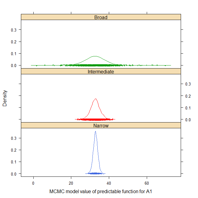
Format
ysimulated response
repreplicate, 4 levels
bsub-plot, 2 levels
awhole-plot, 3 levels
Used with permission of Walt Stroup.
Source
Walter W. Stroup, 1989. Predictable functions and prediction space in the mixed model procedure. Applications of Mixed Models in Agriculture and Related Disciplines.
References
Wolfinger, R.D. and Kass, R.E., 2000. Nonconjugate Bayesian analysis of variance component models, Biometrics, 56, 768–774. https://doi.org/10.1111/j.0006-341X.2000.00768.x
Examples
## Not run:
library(agridat)
data(stroup.splitplot)
dat <- stroup.splitplot
# ---- lme4 ---
# libs(lme4)
# m0 <- lmer(y~ -1 + a + b + a:b + (1|rep) + (1|a:rep), data=dat)
# No predict function
# ----- nlme ---
# libs(nlme)
# m0 <- lme(y ~ -1 + a + b + a:b, data=dat, random = ~ 1|rep/a)
# ----- ASREML model ---
if(require("asreml", quietly=TRUE)){
libs(asreml,lucid)
m1 <- asreml(y~ -1 + a + b + a:b, random=~ rep + a:rep, data=dat)
# vc(m1) # Variance components match Stroup p. 41
## effect component std.error z.ratio bound
## rep 62.42 56.41 1.1 P
## a:rep 15.39 11.8 1.3 P
## units(R) 9.364 4.415 2.1 P
# Narrow space predictions
predict(m1, data=dat, classify="a", average=list(rep=NULL))
# a Predicted Std Err Status
# a1 32.88 1.082 Estimable
# a2 34.12 1.082 Estimable
# a3 25.75 1.082 Estimable
# Intermediate space predictions
predict(m1, data=dat, classify="a", ignore="a:rep",
average=list(rep=NULL))
# a Predicted Std Err Status
# a1 32.88 2.24 Estimable
# a2 34.12 2.24 Estimable
# a3 25.75 2.24 Estimable
# Broad space predictions
predict(m1, data=dat, classify="a")
# a Predicted Std Err Status
# a1 32.88 4.54 Estimable
# a2 34.12 4.54 Estimable
# a3 25.75 4.54 Estimable
}
# ----- MCMCglmm model -----
# Use the point estimates from REML with a prior distribution
libs(lattice,MCMCglmm)
prior2 = list(
G = list(G1=list(V=62.40, nu=1),
G2=list(V=15.38, nu=1)),
R = list(V = 9.4, nu=1)
)
m2 <- MCMCglmm(y~ -1 + a + b + a:b,
random=~ rep + a:rep, data=dat,
pr=TRUE, # save random effects as columns of 'Sol'
nitt=23000, # double the default 13000
prior=prior2, verbose=FALSE)
# posterior.mode(m2$VCV)
# rep a:rep units
# 39.766020 9.617522 7.409334
# plot(m2$VCV)
# Now create a matrix of coefficients for the prediction.
# Each column is for a different prediction. For example,
# the values in the column called 'a1a2n' are multiplied times
# the model coefficients (identified at the right side) to create
# the linear contrast for the the narrow-space predictions
# (also called adjusted mean) for the a1:a2 interaction.
# a1n a1i a1b a1a2n a1a2ib
cm <- matrix(c(1, 1, 1, 1, 1, # a1
0, 0, 0, -1, -1, # a2
0, 0, 0, 0, 0, # a3
1/2, 1/2, 1/2, 0, 0, # b2
0, 0, 0, -1/2, -1/2, # a2:b2
0, 0, 0, 0, 0, # a3:b2
1/4, 1/4, 0, 0, 0, # r1
1/4, 1/4, 0, 0, 0, # r2
1/4, 1/4, 0, 0, 0, # r3
1/4, 1/4, 0, 0, 0, # r4
1/4, 0, 0, 1/4, 0, # a1r1
0, 0, 0, -1/4, 0, # a2r1
0, 0, 0, 0, 0, # a3r1
1/4, 0, 0, 1/4, 0, # a1r2
0, 0, 0, -1/4, 0, # a2r2
0, 0, 0, 0, 0, # a3r2
1/4, 0, 0, 1/4, 0, # a1r3
0, 0, 0, -1/4, 0, # a2r3
0, 0, 0, 0, 0, # a3r3
1/4, 0, 0, 1/4, 0, # a1r4
0, 0, 0, -1/4, 0, # a2r4
0, 0, 0, 0, 0), # a3r4
ncol=5, byrow=TRUE)
rownames(cm) <- c("a1", "a2", "a3", "b2", "a2:b2", "a3:b2",
"r1", "r2", "r3", "r4",
"a1r1", "a1r2", "a1r3", "a1r4", "a2r1", "a2r2",
"a2r3", "a2r4", "a3r1", "a3r2", "a3r3", "a3r4")
colnames(cm) <- c("A1n","A1i","A1b", "A1-A2n", "A1-A2ib")
print(cm)
# post2 <- as.mcmc(m2$Sol
post2 <- as.mcmc(crossprod(t(m2$Sol), cm))
# Following table has columns for A1 estimate (narrow, intermediate, broad)
# A1-A2 estimate (narrow and intermediat/broad).
# The REML estimates are from Stroup 1989.
est <- rbind("REML est"=c(32.88, 32.88, 32.88, -1.25, -1.25),
"REML stderr"=c(1.08, 2.24, 4.54, 1.53, 3.17),
"MCMC mode"=posterior.mode(post2),
"MCMC stderr"=apply(post2, 2, sd))
round(est,2)
# A1n A1i A1b A1-A2n A1-A2ib
# REML est 32.88 32.88 32.88 -1.25 -1.25
# REML stderr 1.08 2.24 4.54 1.53 3.17
# MCMC mode 32.95 32.38 31.96 -1.07 -1.17
# MCMC stderr 1.23 2.64 5.93 1.72 3.73
# plot(post2)
post22 <- lattice::make.groups(
Narrow=post2[,1], Intermediate=post2[,2], Broad=post2[,3])
print(densityplot(~data|which, data=post22, groups=which,
cex=.25, lty=1, layout=c(1,3),
main="stroup.splitplot",
xlab="MCMC model value of predictable function for A1"))
## End(Not run)
Multi-environment trial of barley
Description
Yield for two varieties of barley grown at 51 locations in the years 1901 to 1906.
Format
A data frame with 102 observations on the following 7 variables.
yearyear, 1901-1906
farmerfarmer name
placeplace (nearest town)
districtdistrict, geographical area
gengenotype,
ArcherandGoldthorpeyieldyield, 'stones' per acre (1 stone = 14 pounds)
incomeincome per acre in shillings, based on yield and quality
Details
Experiments were conducted for six years by the Department of Agriculture in Ireland. A total of seven varieties were tested, but only Archer and Goldthorpe were tested in all six years (others were dropped after being found inferior, or were added later). Plots were two acres in size. The value of the grain depended on the yield and quality. Quality varied much from farm to farm, but not so much within the same farm.
The phrase "analysis of variance" first appears in the abstract (only) of a 1918 paper by Fisher. The 1923 paper by Student contained the first analysis of variance table (but not for this data).
One stone is 14 pounds. To convert lb/ac to tonnes/ha, multiply by 0.00112085116
Note: The analysis of Student cannot be reproduced exactly. For example, Student states that the maximum income of Goldthorpe is 230 shillings. A quick glance at Table I of Student shows that the maximum income for Goldthorpe is 220 shillings (11 pounds, 0 shillings) in 1901 at Thurles. Also, the results of Kempton could not be reproduced exactly, perhaps due to rounding or the conversion factor that was used.
Source
Student. 1923. On Testing Varieties of Cereals. Biometrika, 15, 271–293. https://doi.org/10.1093/biomet/15.3-4.271
References
R A Kempton and P N Fox, 1997. Statistical Methods for Plant Variety Evaluation.
Examples
## Not run:
library(agridat)
data(student.barley)
dat <- student.barley
libs(lattice)
bwplot(yield ~ gen|district, dat, main="student.barley - yield")
dat$year <- factor(dat$year)
dat$income <- NULL
# convert to tons/ha
dat <- transform(dat, yield=yield*14 * 0.00112085116)
# Define 'loc' the way that Kempton does
dat$loc <- rep("",nrow(dat))
dat[is.element(dat$farmer, c("Allardyce","Roche","Quinn")),"loc"] <- "1"
dat[is.element(dat$farmer, c("Luttrell","Dooley")), "loc"] <- "2"
dat[is.element(dat$year, c("1904","1905","1906")) & dat$farmer=="Kearney","loc"] <- "2"
dat[dat$farmer=="Mulhall","loc"] <- "3"
dat <- transform(dat, loc=factor(paste(place,loc,sep="")))
libs(reshape2)
datm <- melt(dat, measure.var='yield')
# Kempton Table 9.5
round(acast(datm, loc+gen~year),2)
# Kempton Table 9.6
d2 <- dcast(datm, year+loc~gen)
mean(d2$Archer)
mean(d2$Goldthorpe)
mean(d2$Archer-d2$Goldthorpe)
sqrt(var(d2$Archer-d2$Goldthorpe)/51)
cor(d2$Archer,d2$Goldthorpe)
if(0){
# Kempton Table 9.6b
libs(lme4)
m2 <- lmer(yield~1 + (1|loc) + (1|year) +
(1|loc:year) + (1|gen:loc) + (1|gen:year), data=dat,
control=lmerControl(check.nobs.vs.rankZ="ignore"))
}
## End(Not run)
Uniformity trial of maize, oat, alfalfa, mangolds
Description
Uniformity trial of maize, oat, alfalfa, mangolds
Usage
data("summerby.multi.uniformity")Format
A data frame with 2600 observations on the following 6 variables.
colcolumn ordinate
rowrow ordinate
yieldyield
rangerange (block in field)
yearyear
cropcrop
Details
Note that the plots for each range are the same across years. For example the plots in range R2 are the same in 1922, 1923, 1924, 1925.
Grown at Macdonald College, Quebec. Four ranges of land each 760 x 100 links were used. In years 1922-1926, all crops were harvested in 20 link by 20 links plots.
In oats, the yields are for cleaned grain. In mangolds and alfalfa, the yields of dry matter were calculated. In maize, the green weights of fodder were obtained. In 1925, range R3 oats were damaged by birds. In 1927, range R4 oats were lodges and not harvested. In 1924 range R5 had some flooding and is considered 'inadvisable' for use. In 1914 range R3 oat yield was variable, perhaps from poor germination. Data are included here for completeness, but should perhaps not be included.
The row numbers in this data are based on the figure on page 13 of Summerby. Row 1 is at the bottom. There appears to be approximately a blank row between ranges.
The paper by Summerby has more year/range combinations, but those plots are 20 links by 100 links and are only a single plot wide.
Transcription details: These data were converted from PDF to png images, then OCR converted to text, then hand-checked by K.Wright.
Source
Summerby, R. (1934). The value of preliminary uniformity trials in increasing the precision of field experiments. Macdonald College. https://books.google.com/books?id=6zlMAAAAYAAJ&pg=RA14-PA47
References
None
Examples
## Not run:
library(agridat)
data(summerby.multi.uniformity)
dat <- summerby.multi.uniformity
libs(desplot)
dat <- mutate(dat, env=paste(range, year, crop))
desplot(dat, yield ~ col*row|env, aspect=(5*20)/(35*20),
main="summerby.multi.uniformity")
# Show all ranges for a single year.
# dat
# Compare the variance for each dataset in Summerby, page 18, column (a)
# with what we calculate. Very slight differences.
# libs(dplyr)
# dat
## range year var summerby
## 1 R2 1922 82404 82404
## 2 R2 1923 254780. 254780
## 3 R2 1924 111978. 111978
## 4 R2 1925 84515. 84515
## 5 R2 1926 101008. 100960
## 6 R3 1922 185031. 185031
## 7 R3 1923 154777. 154784
## 8 R3 1924 252451. 252451
## 9 R3 1926 472087. 472088
## 10 R4 1924 19.3 19.341
## 11 R4 1925 14.2 14.234
## 12 R4 1926 14.2 14.236
## 13 R5 1924 134472. 134472
## 14 R5 1925 289001. 289026
## 15 R5 1926 131714. 131714
## 16 R5 1927 8.62 8.622
## End(Not run)
Multi-environment trial of potato
Description
Multi-environment trial of potato tuber yields
Usage
data("tai.potato")Format
A data frame with 48 observations on the following 6 variables.
yieldyield, kg/plot
gengenotype code
varietyvariety name
envenvironment code
loclocation
yearyear
Details
Mean tuber yield of 8 genotypes in 3 locations over two years. Katahdin and Sebago are check varieties. Each location was planted as a 4-rep RCB design.
In Tai's plot of the stability parameters, F5751 and Sebago were in the average stability area. The highest yielding genotype F6032 had an unstable performance.
Source
G.C.C. Tai, 1971. Genotypic stability analysis and its application to potato regional trials. Crop Sci 11, 184-190. Table 2, p. 187. https://doi.org/10.2135/cropsci1971.0011183X001100020006x
References
George Fernandez (1991). Analysis of Genotype x Environment Interaction by Stability Estimates. Hort Science, 26, 947-950.
Examples
## Not run:
library(agridat)
data(tai.potato)
dat <- tai.potato
libs(lattice)
dotplot(variety ~ yield|env, dat, main="tai.potato")
# fixme - need to add tai() example
# note, st4gi::tai assumes there are replications in the data
# https://github.com/reyzaguirre/st4gi/blob/master/R/tai.R
## End(Not run)
Multi-environment trial of potato in UK, yields and trait scores at 12 locations
Description
Yield and 14 trait scores for each of 9 potato varieties at 12 locations in UK.
Usage
data("talbot.potato.traits")
data("talbot.potato.yield")
Format
The talbot.potato.yield dataframe has 126 observations on the following 3 variables.
gengenotype/variety
traittrait
scoretrait score, 1-9
The talbot.potato.yield dataframe has 108 observations on the following 3 variables.
gengenotype/variety
loclocation/center
yieldyield, t/ha
Details
The talbot.potato.yield dataframe contains mean tuber yields
(t/ha) of 9 varieties of potato at 12 centers in the United Kingdom
over five years 1983-1987. The following abbreviations are used for
the centers.
| BU | Bush |
| CA | Cambridge |
| CB | Conon Bridge |
| CC | Crossacreevy |
| CP | Cockle Park |
| CR | Craibstone |
| GR | Greenmount |
| HA | Harper Adams |
| MO | Morley |
| RO | Rosemaund |
| SB | Sutton Bonnington |
| TE | Terrington |
Used with permission of Mike Talbot.
Source
Mike Talbot and A V Wheelwright, 1989, The analysis of genotype x analysis interactions by partial least squares regression. Biuletyn Oceny Odmian, 21/22, 19–25.
Examples
## Not run:
library(agridat)
libs(pls, reshape2)
data(talbot.potato.traits)
datt <- talbot.potato.traits
data(talbot.potato.yield)
daty <- talbot.potato.yield
datt <- acast(datt, gen ~ trait, value.var='score')
daty <- acast(daty, gen ~ loc, value.var='yield')
# Transform columns to zero mean and unit variance
datt <- scale(datt)
daty <- scale(daty)
m1 <- plsr(daty ~ datt, ncomp=3)
summary(m1)
# Loadings factor 1
lo <- loadings(m1)[,1,drop=FALSE]
round(-1*lo[order(-1*lo),1,drop=FALSE],2)
biplot(m1, main="talbot.potato - biplot")
## End(Not run)
Multi-environment trial of millet
Description
Multi-environment trial of millet
Usage
data("tesfaye.millet")Format
A data frame with 415 observations on the following 9 variables.
yearyear
sitesite (location)
repreplicate
colcolumn ordinate
rowrow ordinate
plotplot number
gengenotype
entry_numberentry
yieldyield, kg/ha
Details
Experiments conducted at Bako and Assosa research centers in Ethiopia. The data has: 4 years, 2 sites = 7 environments, 2-3 reps per trial, 47 genotypes.
Tesfaye et al used asreml to fit a GxE model with Factor Analytic covariance structure for the GxE part and AR1xAR1 for spatial residuals at each site.
Data in PloS ONE was published under Creative Commons Attribution License.
Source
Tesfaye K, Alemu T, Argaw T, de Villiers S, Assefa E (2023) Evaluation of finger millet (Eleusine coracana (L.) Gaertn.) in multi-environment trials using enhanced statistical models. PLoS ONE 18(2): e0277499. https://doi.org/10.1371/journal.pone.0277499
References
None
Examples
## Not run:
library(agridat)
data(tesfaye.millet)
dat <- tesfaye.millet
dat <- transform(dat, year=factor(year), site=factor(site))
libs(dplyr,asreml,lucid)
dat <- mutate(dat,
env=factor(paste0(site,year)),
gen=factor(gen),
rep=factor(rep),
xfac=factor(col), yfac=factor(row))
libs(desplot)
desplot(dat, yield~col*row|env, main="tesfaye.millet")
dat <- arrange(dat, env, xfac, yfac)
# Fixed environment
# Random row/col within environment, Factor Analytic GxE
# AR1xAR1 spatial residuals within each environment
if(require("asreml", quietly=TRUE)){
libs(asreml)
m1 <- asreml(yield ~ 1 + env,
data=dat,
random = ~ at(env):xfac + at(env):yfac + gen:fa(env),
residual = ~ dsum( ~ ar1(xfac):ar1(yfac)|env) )
m1 <- update(m1)
lucid::vc(m1)
}
## End(Not run)
Multi-environment trial of barley, multiple years & fertilizer levels
Description
Barley yields at multiple locs, years, fertilizer levels
Usage
data("theobald.barley")Format
A data frame with 105 observations on the following 5 variables.
yieldyield, tonnes/ha
gengenotype
loclocation, 5 levels
nitronitrogen kg/ha
yearyear, 2 levels
Details
Theobald and Talbot used BUGS to fit a fully Bayesian model for yield response curves.
Locations of the experiment were in north-east Scotland.
Assumed nitrogen cost 400 pounds per tonne. Grain prices used were 100, 110, and 107.50 pounds per tonne for Georgie, Midas and Sundance.
Source
Chris M. Theobald and Mike Talbot, (2002). The Bayesian choice of crop variety and fertilizer dose. Appl Statistics, 51, 23-36. https://doi.org/10.1111/1467-9876.04863
Data provided by Chris Theobald and Mike Talbot.
Examples
## Not run:
library(agridat)
data(theobald.barley)
dat <- theobald.barley
dat <- transform(dat, env=paste(loc,year,sep="-"))
dat <- transform(dat, income=100*yield - 400*nitro/1000)
libs(lattice)
xyplot(income~nitro|env, dat, groups=gen, type='b',
auto.key=list(columns=3), main="theobald.barley")
## End(Not run)
Multi-environment trial of corn silage, Year * Loc * Variety with covariate
Description
Corn silage yields for maize in 5 years at 7 districts for 10 hybrids.
Format
A data frame with 256 observations on the following 5 variables.
yearyear, 1990-1994
envenvironment/district, 1-7
gengenotype, 1-10
yielddry-matter silage yield for corn
chucorn heat units, thousand degrees Celsius
Used with permission of Chris Theobald.
Details
The trials were carried out in seven districts in the maritime provinces of Eastern Canada. Different fields were used in successive years. The covariate CHU (Corn Heat Units) is the accumulated average daily temperatures (thousands of degrees Celsius) during the growing season at each location.
Source
Chris M. Theobald and Mike Talbot and Fabian Nabugoomu, 2002. A Bayesian Approach to Regional and Local-Area Prediction From Crop Variety Trials. Journ Agric Biol Env Sciences, 7, 403–419. https://doi.org/10.1198/108571102230
Examples
## Not run:
library(agridat)
data(theobald.covariate)
dat <- theobald.covariate
libs(lattice)
xyplot(yield ~ chu|gen, dat, type=c('p','smooth'),
xlab = "chu = corn heat units",
main="theobald.covariate - yield vs heat")
# REML estimates (Means) in table 3 of Theobald 2002
libs(lme4)
dat <- transform(dat, year=factor(year))
m0 <- lmer(yield ~ -1 + gen + (1|year/env) + (1|gen:year), data=dat)
round(fixef(m0),2)
# Use JAGS to fit Theobald (2002) model 3.2 with 'Expert' prior
# Requires JAGS to be installed
if(0) {
libs(reshape2)
ymat <- acast(dat, year+env~gen, value.var='yield')
chu <- acast(dat, year+env~., mean, value.var='chu', na.rm=TRUE)
chu <- as.vector(chu - mean(chu)) # Center the covariate
dat$yr <- as.numeric(dat$year)
yridx <- as.vector(acast(dat, year+env~., mean, value.var='yr', na.rm=TRUE))
dat$loc <- as.numeric(dat$env)
locidx <- acast(dat, year+env~., mean, value.var='loc', na.rm=TRUE)
locidx <- as.vector(locidx)
jdat <- list(nVar = 10, nYear = 5, nLoc = 7, nYL = 29, yield = ymat,
chu = chu, year = yridx, loc = locidx)
libs(rjags)
m1 <- jags.model(file=system.file(package="agridat", "files/theobald.covariate.jag"),
data=jdat, n.chains=2)
# Table 3, Variety deviations from means (Expert prior)
c1 <- coda.samples(m1, variable.names=(c('alpha')),
n.iter=10000, thin=10)
s1 <- summary(c1)
effs <- s1$statistics[,'Mean']
# Perfect match (different order?)
rev(sort(round(effs - mean(effs), 2)))
}
## End(Not run)
Multi-environment trial of corn & soybean, 1930-1962, with temperature and precipitation
Description
Average yield of corn and soybeans in five U.S. states (IA, IL, IN, MO, OH) during the years 1930-1962. Pre-season precipitation and average temperature and precipitation during each month of the growing season is included.
Format
statestate
yearyear, 1930-1962
rain0pre-season precipitation in inches
temp5may temperature, Fahrenheit
rain6june rain, inches
temp6june temp
rain7july rain
temp7july temp
rain8august rain
temp8august temp
corncorn yield, bu/acre
soysoybean yield, bu/acre
Details
Note: The Iowa corn data has sometimes been identified (in other sources) as the "Iowa wheat" data, but this is incorrect.
The 'year' variable affects yield through (1) improvements in plant genetics (2) changes in management techniques such as fertilizer, chemicals, tillage, planting date, and (3) climate, pest infestations, etc.
Double-cross corn hybrids were introduced in the 1920s. Single-cross hybrids became common around 1960.
During World War II, nitrogen was used in the production of TNT for bombs. After the war, these factories switched to producing ammonia for fertilizer. Nitrogen fertilizer use greatly increased after WWII and is a major reason for yield gains of corn. Soybeans gain little benefit from nitrogen fertilizer. The other major reason for increasing yields in both crops is due to improved plant genetics.
Crops are often planted in May, and harvest begins in September.
Yields in 1936 were very low due to July being one of the hottest and driest on record.
Some relevant maps of yield, heat, and precipitation can be found in Atlas of crop yield and summer weather patterns, 1931-1975, https://www.isws.illinois.edu/pubdoc/C/ISWSC-150.pdf
The following notes pertain to the Iowa data.
The 1947 June precipitation of 10.33 inches was the wettest June on record (a new Iowa June record of 10.34 inches was set in 2010). As quoted in Monthly Weather Review (Dec 1957, p. 396) "The dependence of Iowa agriculture upon the vagaries of the weather was closely demonstrated during the 1947 season. A cool wet spring delayed crop planting activity and plant growth; then, in addition, a hard freeze on May 29th ... further set back the corn. The heavy rains and subsequent floods during June caused appreciable crop acreage to be abandoned ... followed by a hot dry weather regime that persisted from mid-July through the first week of September."
In 1949 soybean yields were average while corn yields were low. From the same source above, "The year 1949 saw the greatest infestation of corn borer in the history of corn in Iowa".
1955 yields were reduced due to dry weather in late July and August.
Source
Thompson, L.M., 1963. Weather and technology in the production of corn and soybeans. CAED Report 17. The Center for Agriculture and Economic Development, Iowa State University, Ames, Iowa.
References
Draper, N. R. and Smith, H. (1981). Applied Regression Analysis, second ed., Wiley, New York.
Examples
## Not run:
library(agridat)
data(thompson.cornsoy)
dat <- thompson.cornsoy
# The droughts of 1934/36 were severe in IA/MO. Less so in OH.
libs(lattice)
xyplot(corn+soy~year|state, dat,
type=c('p','l','r'), auto.key=list(columns=2),
main="thompson.cornsoy",
layout=c(5,1),ylab='yield')
# In 1954, only Missouri suffered very hot, dry weather
## xyplot(corn~year, dat,
## groups=state, type=c('p','l'),
## main="thompson.cornsoy",
## auto.key=list(columns=5), ylab='corn yield')
# Rain and temperature have negative correlation in each month.
# July is a critical month: temp and yield are negatively correlated,
# while rain and yield are positively correlated.
# splom(~dat[-1,-1], col=dat$state, cex=.5, main="thompson.cornsoy")
# Plots similar to those in Venables' Exegeses paper.
dat.ia <- subset(dat, state=="Iowa")
libs(splines)
m2 <- aov(corn ~ ns(rain0, 3) + ns(rain7, 3) +
ns(temp8, 3) + ns(year,3), dat.ia)
op <- par(mfrow=c(2,2))
termplot(m2, se=TRUE, rug=TRUE, partial=TRUE, main="thompson.cornsoy")
par(op)
# do NOT use gam package
libs(mgcv)
m1 <- gam(corn ~ s(year, k=5) + s(rain0, k=5) +
s(rain7, k=5) + s(temp8, k=5), data=dat.ia)
op <- par(mfrow=c(2,2))
plot.gam(m1, residuals=TRUE, se=TRUE, cex=2, main="thompson.cornsoy")
par(op)
## End(Not run)
Uniformity trial of winter/spring wheat
Description
Uniformity trial of winter/spring wheat in Russia
Usage
data("tulaikow.wheat.uniformity")Format
A data frame with 480 observations on the following 4 variables.
rowrow ordinate
colcolumn ordinate
yieldyield in grams per plot
seasonwinter or summer
Details
Land was fallow in 1911, harvested in 1912 at the Bezenchuk Experimental Station in Russia. A winter wheat field of 240 square sazhen (24 x 10 sazhen) was divided into separate plots of 1 square sazhen, which were cut, threshed and weighed separately.
In the same way, a plot of Poltavka spring wheat was harvested and a plot of 240 square sazhen with dimensions of 15 by 16 sazhen was divided into plots of 1 square sazhen.
Winter wheat:
Field length: 10 rows * 1 sazhen.
Field width: 24 columns * 1 sazhen.
Summer wheat:
Field length: 16 rows * 1 sazhen.
Field width: 15 columns * 1 sazhen.
Note: The Russian word (that looks like "cax" with a vertical line in the "x") refers to a unit of measurement. Specifically, it represents the sazhen, which was used in traditional Russian systems of measurement. The sazhen itself is approximately 3 meters (7 feet) long. Google Translate sometimes converts "sazhen" into "soot", "meter" or "fathom".
Transcription details: The data were typed by K.Wright from Roemer (1920), table 4, p. 63.
Source
N. Tulaikow (1913) Resultate einer mathematischen Bearbeitung von Ernteergebnissen. Russian Journal fur Exp Landw., 14, 88-113. https://www.google.com/books/edition/Journal_de_l_agriculture_experimentale/i2EjAQAAIAAJ?hl=en&gbpv=1&dq=tulaikow
References
Neyman, J., & Iwaszkiewicz, K. (1935). Statistical problems in agricultural experimentation. Supplement to the Journal of the Royal Statistical Society, 2(2), 107-180.
Roemer, T. (1920). Der Feldversuch. Arbeiten der Deutschen Landwirtschafts-Gesellschaft, 302. https://www.google.com/books/edition/Arbeiten_der_Deutschen_Landwirtschafts_G/7zBSAQAAMAAJ
Examples
## Not run:
library(agridat)
data(tulaikow.wheat.uniformity)
dat <- tulaikow.wheat.uniformity
libs(desplot)
desplot(dat, yield~col*row, subset=season=="winter",
aspect=10/24, flip=TRUE, tick=TRUE,
main="tulaikow.wheat.uniformity (winter)")
desplot(dat, yield~col*row, subset=season=="summer",
aspect=16/15, flip=TRUE, tick=TRUE,
main="tulaikow.wheat.uniformity (summer)")
## End(Not run)
Herbicide control of larkspur
Description
Herbicide control of larkspur
Usage
data("turner.herbicide")Format
A data frame with 12 observations on the following 4 variables.
reprep factor
raterate of herbicide
livenumber of live plants before application
deadnumber of plants killed by herbicide
Details
Effectiveness of the herbicide Picloram on larkspur plants at 4 doses (0, 1.1, 2.2, 4.5) in 3 reps. Experiment was done in 1986 at Manti, Utah.
Source
David L. Turner and Michael H. Ralphs and John O. Evans (1992). Logistic Analysis for Monitoring and Assessing Herbicide Efficacy. Weed Technology, 6, 424-430. https://www.jstor.org/stable/3987312
References
Christopher Bilder, Thomas Loughin. Analysis of Categorical Data with R.
Examples
## Not run:
library(agridat)
data(turner.herbicide)
dat <- turner.herbicide
dat <- transform(dat, prop=dead/live)
# xyplot(prop~rate,dat, pch=20, main="turner.herbicide", ylab="Proportion killed")
m1 <- glm(prop~rate, data=dat, weights=live, family=binomial)
coef(m1) # -3.46, 2.6567 Same as Turner eqn 3
# Make conf int on link scale and back-transform
p1 <- expand.grid(rate=seq(0,to=5,length=50))
p1 <- cbind(p1, predict(m1, newdata=p1, type='link', se.fit=TRUE))
p1 <- transform(p1, lo = plogis(fit - 2*se.fit),
fit = plogis(fit),
up = plogis(fit + 2*se.fit))
# Figure 2 of Turner
libs(latticeExtra)
foo1 <- xyplot(prop~rate,dat, cex=1.5,
main="turner.herbicide (model with 2*S.E.)",
xlab="Herbicide rate", ylab="Proportion killed")
foo2 <- xyplot(fit~rate, p1, type='l')
foo3 <- xyplot(lo+up~rate, p1, type='l', lty=1, col='gray')
print(foo1 + foo2 + foo3)
# What dose gives a LD90 percent kill rate?
# libs(MASS)
# dose.p(m1, p=.9)
## Dose SE
## p = 0.9: 2.12939 0.128418
# Alternative method
# libs(car) # logit(.9) = 2.197225
# deltaMethod(m1, g="(log(.9/(1-.9))-b0)/(b1)", parameterNames=c('b0','b1'))
## Estimate SE
## (2.197225 - b0)/(b1) 2.12939 0.128418
# What is a 95 percent conf interval for LD90? Bilder & Loughin page 138
root <- function(x, prob=.9, alpha=0.05){
co <- coef(m1) # b0,b1
covs <- vcov(m1) # b00,b11,b01
# .95 = b0 + b1*x
# (b0+b1*x) + Z(alpha/2) * sqrt(b00 + x^2*b11 + 2*x*b01) > .95
# (b0+b1*x) - Z(alpha/2) * sqrt(b00 + x^2*b11 + 2*x*b01) < .95
f <- abs(co[1] + co[2]*x - log(prob/(1-prob))) /
sqrt(covs[1,1] + x^2 * covs[2,2] + 2*x*covs[1,2])
return( f - qnorm(1-alpha/2))
}
lower <- uniroot(f=root, c(0,2.13))
upper <- uniroot(f=root, c(2.12, 5))
c(lower$root, upper$root)
# 1.92 2.45
## End(Not run)
Weight gain calves in a feedlot
Description
Weight gain calves in a feedlot, given three different diets.
Usage
data("urquhart.feedlot")Format
A data frame with 67 observations on the following 5 variables.
animalanimal ID
herdherd ID
dietdiet: Low, Medium, High
weight1initial weight
weight2slaughter weight
Details
Calves born in 1975 in 11 different herds entered a feedlot as yearlings. Each animal was fed one of three diets with low, medium, or high energy. The original sources explored the use of some contrasts for comparing breeds.
| Herd | Breed |
| 9 | New Mexico Herefords |
| 16 | New Mexico Herefords |
| 3 | Utah State University Herefords |
| 32 | Angus |
| 24 | Angus x Hereford (cross) |
| 31 | Charolais x Hereford |
| 19 | Charolais x Hereford |
| 36 | Charolais x Hereford |
| 34 | Brangus |
| 35 | Brangus |
| 33 | Southern Select |
Source
N. Scott Urquhart (1982). Adjustment in Covariance when One Factor Affects the Covariate Biometrics, 38, 651-660. Table 4, p. 659. https://doi.org/10.2307/2530046
References
N. Scott Urquhart and David L. Weeks (1978). Linear Models in Messy Data: Some Problems and Alternatives Biometrics, 34, 696-705. https://doi.org/10.2307/2530391
Also available in the 'emmeans' package as the 'feedlot' data.
Examples
## Not run:
library(agridat)
data(urquhart.feedlot)
dat <- urquhart.feedlot
libs(reshape2)
d2 <- melt(dat, id.vars=c('animal','herd','diet'))
libs(latticeExtra)
useOuterStrips(xyplot(value ~ variable|diet*herd, data=d2, group=animal,
type='l',
xlab="Initial & slaughter timepoint for each diet",
ylab="Weight for each herd",
main="urquhart.feedlot - weight gain by animal"))
# simple fixed-effects model
dat <- transform(dat, animal = factor(animal), herd=factor(herd))
m1 <- lm(weight2 ~ weight1 + herd*diet, data = dat)
coef(m1) # weight1 = 1.1373 match Urquhart table 5 common slope
# random-effects model might be better, for example
# libs(lme4)
# m1 <- lmer(weight2 ~ -1 + diet + weight1 + (1|herd), data=dat)
# summary(m1) # weight1 = 1.2269
## End(Not run)
Adoption of genetically modified crops in the United States
Description
Adoption of genetically modified crops in the U.S. from 1996 to 2022.
Usage
data("usda.gmoadoption")Format
A data frame with 145 observations on the following 3 variables.
yearYear of crop
cropCrop type
percentPercent of planted acres
Details
HT indicates herbicide-tolerant crops. Bt indicates insect-resistant (Bacillus thuringiensis) crops. The "percent" column is the percentage of planted acres for each crop that were genetically modified. HT/Bt for corn and cotton are not mutually exclusive categories. For example, as time progressed corn hybrids tended to be both HT and Bt.
Source
Adoption of Genetically Engineered Crops in the United States - Recent Trends in GE Adoption USDA Economic Research Service. Accessed 2025-09-30. https://www.ers.usda.gov/data-products/adoption-of-genetically-engineered-crops-in-the-united-states/recent-trends-in-ge-adoption
References
None
Examples
## Not run:
data(usda.gmoadoption)
dat <- usda.gmoadoption
library(ggplot2)
ggplot(dat, aes(x = year, y = percent, color = crop)) +
geom_point() +
geom_line() +
labs(
title = "Adoption of Genetically Engineered Crops in the U.S.",
y = "Percentage of acres for each crop"
) +
theme_minimal()
## End(Not run)
Concentrations of herbicides in streams in the United States
Description
Concentrations of selected herbicides and degradation products determined by laboratory method analysis code GCS for water samples collected from 51 streams in nine Midwestern States, 2002.
Usage
data("usgs.herbicides")Format
A data frame with 184 observations on the following 19 variables.
mapnummap number
usgsidUSGS ID
longlongitude
latlatitude
sitesite name
citycity
sampletypesample type code
datedate sample was collected
hourhour sample was collected
acetochlorconcentration as character
alachlorconcentration as character
ametrynconcentration as character
atrazineconcentration as character
CIATconcentration as character
CEATconcentration as character
cyanazineconcentration as character
CAMconcentration as character
dimethenamidconcentration as character
flufenacetconcentration as character
Details
Concentrations of selected herbicides and degradation products determined by laboratory method analysis code GCS for water samples collected from 51 streams in nine Midwestern States, 2002.
All concentrations are micrograms/liter, "<" means "less than". The data are in character format to allow for "<".
The original report contains data for more herbicides. This data is for illustrative purposes.
Sample types: CR = concurrent replicate sample, FB = field blank, LD = laboratory duplicate, S1 = sample from pre-emergence runoff, S2 = sample from post-emergence runoff, S3 = sample from harvest-season runoff.
Source
Scribner, E.A., Battaglin, W.A., Dietze, J.E., and Thurman, E.M., "Reconnaissance Data for Glyphosate, Other Selected Herbicides, their Degradation Products, and Antibiotics in 51 streams in Nine Midwestern States, 2002". U.S. Geological Survey Open File Report 03-217. Herbicide data from table 5, page 30-37. Site coordinates page 7-8. https://ks.water.usgs.gov/pubs/reports/ofr.03-217.html
References
None.
Examples
## Not run:
library(agridat)
data(usgs.herbicides)
dat <- usgs.herbicides
# create censored data for one trait
dat$y <- as.numeric(dat$atrazine)
dat$ycen <- is.na(dat$y)
dat$y[is.na(dat$y)] <- .05
# library(NADA)
# # percent censored
# with(dat, censummary(y, censored=ycen))
# # median/mean
# with(dat, cenmle(y, ycen, dist="lognormal"))
# # boxplot
# with(dat, cenboxplot(obs=y, cen=ycen, log=FALSE,
# main="usgs.herbicides"))
# # with(dat, boxplot(y))
# pp <- with(dat, ros(obs=y, censored=ycen, forwardT="log")) # default lognormal
# plot(pp)
# plotfun <- function(vv){
# dat$y <- as.numeric(dat[[vv]])
# dat$ycen <- is.na(dat$y)
# dat$y[is.na(dat$y)] <- .01
# # qqnorm(log(dat$y), main=vv) # ordinary qq plot shows censored values
# pp <- with(dat, ros(obs=y, censored=ycen, forwardT="log"))
# plot(pp, main=vv) # omits censored values
# }
# op <- par(mfrow=c(3,3))
# vnames <- c("acetochlor", "alachlor", "ametryn", "atrazine","CIAT", "CEAT", "cyanazine", #"CAM",
# "dimethenamid", "flufenacet")
# for(vv in vnames) plotfun(vv)
# par(op)
## End(Not run)
Multi-environment trial of maize, dry matter content
Description
Multi-environment trial of maize, dry matter content
Usage
data("vaneeuwijk.drymatter")Format
A data frame with 168 observations on the following 5 variables.
yearyear
sitesite, 4 levels
varietyvariety, 6 levels
ydry matter percent
Details
Percent dry matter is given.
Site codes are soil type classifications: SS=Southern Sand, CS=Central Sand, NS=Northern Sand, RC=River Clay.
These data are a balanced subset of the data analyzed in van Eeuwijk, Keizer, and Bakker (1995b) and Kroonenberg, Basford, and Ebskamp (1995).
Used with permission of Fred van Eeuwijk.
Source
van Eeuwijk, Fred A. and Pieter M. Kroonenberg (1998). Multiplicative Models for Interaction in Three-Way ANOVA, with Applications to Plant Breeding Biometrics, 54, 1315-1333. https://doi.org/10.2307/2533660
References
Kroonenberg, P.M., Basford, K.E. & Ebskamp, A.G.M. (1995). Three-way cluster and component analysis of maize variety trials. Euphytica, 84(1):31-42. https://doi.org/10.1007/BF01677554
van Eeuwijk, F.A., Keizer, L.C.P. & Bakker, J.J. Van Eeuwijk. (1995b). Linear and bilinear models for the analysis of multi-environment trials: II. An application to data from the Dutch Maize Variety Trials Euphytica, 84(1):9-22. https://doi.org/10.1007/BF01677552
Hardeo Sahai, Mario M. Ojeda. Analysis of Variance for Random Models, Volume 1. Page 261.
Examples
## Not run:
library(agridat)
data(vaneeuwijk.drymatter)
dat <- vaneeuwijk.drymatter
dat <- transform(dat, year=factor(year))
dat <- transform(dat, env=factor(paste(year,site)))
libs(HH)
HH::interaction2wt(y ~ year+site+variety,dat,rot=c(90,0),
x.between=0, y.between=0,
main="vaneeuwijk.drymatter")
# anova model
m1 <- aov(y ~ variety+env+variety:env, data=dat)
anova(m1) # Similar to VanEeuwijk table 2
m2 <- aov(y ~ year*site*variety, data=dat)
anova(m2) # matches Sahai table 5.5
# variance components model
libs(lme4)
libs(lucid)
m3 <- lmer(y ~ (1|year) + (1|site) + (1|variety) +
(1|year:site) + (1|year:variety) + (1|site:variety),
data=dat)
vc(m3) # matches Sahai page 266
## grp var1 var2 vcov sdcor
## year:variety (Intercept) <NA> 0.3187 0.5645
## year:site (Intercept) <NA> 7.735 2.781
## site:variety (Intercept) <NA> 0.03502 0.1871
## year (Intercept) <NA> 6.272 2.504
## variety (Intercept) <NA> 0.4867 0.6976
## site (Intercept) <NA> 6.504 2.55
## Residual <NA> <NA> 0.8885 0.9426
## End(Not run)
Infection of wheat varieties by Fusarium strains from 1990 to 1993
Description
Infection of wheat varieties by Fusarium strains from 1990 to 1993
Usage
data("vaneeuwijk.fusarium")Format
A data frame with 560 observations on the following 4 variables.
yearyear, 1990-1993
strainstrain of fusarium
gengenotype/variety
y
Details
Data come from Hungary. There were 20 wheat varieties infected with 7 strains of Fusarium in the years 1990-1993. The measured value is a rating of the severity of disease due to Fusarium head blight, expressed as a number 1-100.
Three-way interactions for varieties 21 and 23 were the only ones in 1992 suffering from strain infections. This was due to incorrect storage of the innoculum (strain) which rendered it incapable of infecting most other varieties.
The data is a subset of the data analyzed by VanEeuwijk et al. 1995.
Used with permission of Fred van Eeuwijk.
Source
van Eeuwijk, Fred A. and Pieter M. Kroonenberg (1998). Multiplicative Models for Interaction in Three-Way ANOVA, with Applications to Plant Breeding Biometrics, 54, 1315-1333. https://doi.org/10.2307/2533660
References
F. A. van Eeuwijk, A. Mesterhazy, Ch. I. Kling, P. Ruckenbauer, L. Saur, H. Burstmayr, M. Lemmens, L. C. P. Keizer, N. Maurin, C. H. A. Snijders. (1995). Assessing non-specificity of resistance in wheat to head blight caused by inoculation with European strains of Fusarium culmorum, F. graminearum and F. nivale using a multiplicative model for interaction. Theor Appl Genet. 90(2), 221-8. https://doi.org/10.1007/BF00222205
Examples
## Not run:
library(agridat)
data(vaneeuwijk.fusarium)
dat <- vaneeuwijk.fusarium
dat <- transform(dat, year=factor(year))
dat <- transform(dat, logity=log((y/100)/(1-y/100)))
libs(HH)
position(dat$year) <- c(3,9,14,19)
position(dat$strain) <- c(2,5,8,11,14,17,20)
HH::interaction2wt(logity ~ gen+year+strain,dat,rot=c(90,0),
x.between=0, y.between=0,
main="vaneeuwijk.fusarium")
# anova on logit scale. Near match to VanEeuwijk table 6
m1 <- aov(logity ~ gen*strain*year, data=dat)
anova(m1)
## Response: logity
## Df Sum Sq Mean Sq F value Pr(>F)
## gen 19 157.55 8.292
## strain 6 91.54 15.256
## year 3 321.99 107.331
## gen:strain 114 34.03 0.299
## gen:year 57 140.94 2.473
## strain:year 18 236.95 13.164
## gen:strain:year 342 93.15 0.272
## End(Not run)
Number of cysts on 11 potato genotypes for 5 potato cyst nematode populations.
Description
The number of cysts on 11 potato genotypes for 5 potato cyst nematode populations.
Usage
data("vaneeuwijk.nematodes")Format
A data frame with 55 observations on the following 3 variables.
genpotato genotype
popnematode population
ynumber of cysts
Details
The number of cysts on 11 potato genotypes for 5 potato cyst nematode populations belonging to the species Globodera pallida. This is part of a larger table in . The numbers are the means over four or five replicates.
Van Eeuwijk used this data to illustrate fitting a generalized linear model.
Source
Fred A. van Eeuwijk, (1995). Multiplicative Interaction in Generalized Linear Models. Biometrics, 51, 1017-1032. https://doi.org/10.2307/2533001
References
Arntzen, F.K. & van Eeuwijk (1992). Variation in resistance level of potato genotypes and virulence level of potato cyst nematode populations. Euphytica, 62, 135-143. https://doi.org/10.1007/BF00037939
Examples
## Not run:
library(agridat)
data(vaneeuwijk.nematodes)
dat <- vaneeuwijk.nematodes
# show non-normality
op <- par(mfrow=c(2,1), mar=c(5,4,3,2))
boxplot(y ~ pop, data=dat, las=2,
ylab="number of cysts")
title("vaneeuwijk.nematodes - cysts per nematode pop")
boxplot(y ~ gen, data=dat, las=2)
title("vaneeuwijk.nematodes - cysts per potato")
par(op)
# normal distribution
lm1 <- lm(y ~ gen + pop, data=dat)
# poisson distribution
glm1 <- glm(y ~ gen+pop,data=dat,family=quasipoisson(link=log))
anova(glm1)
libs(gnm)
# main-effects non-interaction model
gnm0 <- gnm(y ~ pop + gen, data=dat,
family=quasipoisson(link=log))
# one interaction
gnm1 <- gnm(y ~ pop + gen + Mult(pop,gen,inst=1), data=dat,
family=quasipoisson(link=log))
# two interactions
gnm2 <- gnm(y ~ pop + gen + Mult(pop,gen,inst=1) + Mult(pop,gen,inst=2),
data=dat,
family=quasipoisson(link=log))
# anova(gnm0, gnm1, gnm2, test="F")
# only 2, not 3 axes needed
# match vaneeuwijk table 2
# anova(gnm2)
## Df Deviance Resid. Df Resid. Dev
## NULL 54 8947.4
## pop 4 690.6 50 8256.8
## gen 10 7111.4 40 1145.4
## Mult(pop, gen, inst = 1) 13 716.0 27 429.4
## Mult(pop, gen, inst = 2) 11 351.1 16 78.3
# compare residual qq plots from models
op <- par(mfrow=c(2,2))
plot(lm1, which=2, main="LM")
plot(glm1, which=2, main="GLM")
plot(gnm0, which=2, main="GNM, no interaction")
plot(gnm2, which=2, main="GNM, 2 interactions")
par(op)
# extract interaction-term coefficients, make a biplot
pops <- pickCoef(gnm2, "[.]pop")
gens <- pickCoef(gnm2, "[.]gen")
coefs <- coef(gnm2)
A <- matrix(coefs[pops], nc = 2)
B <- matrix(coefs[gens], nc = 2)
A2=scale(A)
B2=scale(B)
rownames(A2) <- levels(dat$pop)
rownames(B2) <- levels(dat$gen)
# near-match with vaneeuwijk figure 1
biplot(A2,B2, expand=2.5,xlim=c(-2,2),ylim=c(-2,2),
main="vaneeuwijk.nematodes - GAMMI biplot")
## End(Not run)
Treatment x environment interaction in agronomy trials
Description
Treatment x environment interaction in agronomy trials
Usage
data("vargas.txe.covs")
data("vargas.txe.yield")
Format
The 'vargas.txe.covs' data has 10 years of measurements on 28 environmental covariates:
yearyear
MTDmean maximum temperature in December
MTJmean maximum temperature in January
MTFmean maximum temperature in February
MTMmean maximum temperature in March
MTAmean maximum temperature in April
mTDmean minimum temperature in December
mTJmean minimum temperature in January
mTFmean minimum temperature in February
mTMmean minimum temperature in March
mTAmean minimum temperature in April
mTUDmean minimum temperature in December
mTUJmean minimum temperature in January
mTUFmean minimum temperature in February
mTUMmean minimum temperature in March
mTUAmean minimum temperature in April
PRDtotal monthly precipitation in December
PRJtotal monthly precipitation in Jan
PRFtotal monthly precipitation in Feb
PRMtotal monthly precipitation in Mar
SHDsun hours per day in Dec
SHJsun hours per day in Jan
SHFsun hours per day in Feb
EVDtotal monthly evaporation in Dec
EVJtotal monthly evaporation in Jan
EVFtotal monthly evaporation in Feb
EVMtotal monthly evaporation in Mar
EVAtotal monthly evaporation in Apr
The 'vargas.txe.yield' dataframe contains 240 observations on three variables
yearYear
trtTreatment. See details section
yieldGrain yield, kg/ha
Details
The treatment names indicate:
| T | deep knife |
| t | no deep knife |
| S | sesbania |
| s | soybean |
| M | chicken manure |
| m | no chicken manure |
| 0 | no nitrogen |
| n | 100 kg/ha nitrogen |
| N | 200 kg/ha nitrogen |
Used with permission of Jose Crossa.
Source
Vargas, Mateo and Crossa, Jose and van Eeuwijk, Fred and Sayre, Kenneth D. and Reynolds, Matthew P. (2001). Interpreting Treatment x Environment Interaction in Agronomy Trials. Agron. J., 93, 949-960. Table A1, A3. https://doi.org/10.2134/agronj2001.934949x
Examples
## Not run:
library(agridat)
data(vargas.txe.covs)
data(vargas.txe.yield)
libs(reshape2)
libs(lattice)
redblue <- colorRampPalette(c("firebrick", "lightgray", "#375997"))
Z <- vargas.txe.yield
Z <- acast(Z, year ~ trt, value.var='yield')
levelplot(Z, col.regions=redblue,
main="vargas.txe.yield", xlab="year", ylab="treatment",
scales=list(x=list(rot=90)))
# Double-centered like AMMI
Z <- sweep(Z, 1, rowMeans(Z))
Z <- sweep(Z, 2, colMeans(Z))
# Vargas figure 1
biplot(prcomp(Z, scale.=FALSE), main="vargas.txe.yield")
# Now, PLS relating the two matrices
U <- vargas.txe.covs
U <- scale(U) # Standardized covariates
libs(pls)
m1 <- plsr(Z~U)
# Vargas Fig 2, flipped vertical/horizontal
biplot(m1, which="x", var.axes=TRUE)
## End(Not run)
Wheat yields in 7 years with genetic and environment covariates
Description
Yield of Durum wheat, 7 genotypes, 6 years, with 16 genotypic variates and 16 environment variates.
Usage
data("vargas.wheat1.covs")
data("vargas.wheat1.traits")
Format
The vargas.wheat1.covs dataframe has 6 observations on the following 17 variables.
yearyear, 1990-1995
MTDMean daily max temperature December, deg C
MTJMean max in January
MTFMean max in February
MTMMean max in March
mTDMean daily minimum temperature December, deg C
mTJMean min in January
mTFMean min in February
mTMMean min in March
PRDMonthly precipitation in December, mm
PRJPrecipitation in January
PRFPrecipitation in February
PRMPrecipitation in March
SHDSun hours in December
SHJSun hours in January
SHFSun hours in February
SHMSun hours in March
The vargas.wheat1.traits dataframe has 126 observations on the following 19 variables.
yearyear, 1990-1995
repreplicate, 3 levels
gengenotype, 7 levels
yieldyield, kg/ha
ANTanthesis, days after emergence
MATmaturity, days after emergence
GFIgrainfill, MAT-ANT
PLHplant height, cm
BIObiomass above ground, kg/ha
HIDharvest index
STWstraw yield, kg/ha
NSMspikes / m^2
NGMgrains / m^2
NGSgrains per spike
TKWthousand kernel weight, g
WTIweight per tiller, g
SGWspike grain weight, g
VGRvegetative growth rate, kg/ha/day, STW/ANT
KGRkernel growth rate, mg/kernel/day
Details
Conducted in Ciudad Obregon, Mexico.
Source
Mateo Vargas and Jose Crossa and Ken Sayre and Matthew Renolds and Martha E Ramirez and Mike Talbot, 1998. Interpreting Genotype x Environment Interaction in Wheat by Partial Least Squares Regression. Crop Science, 38, 679-689. https://doi.org/10.2135/cropsci1998.0011183X003800030010x
Data provided by Jose Crossa.
Examples
## Not run:
library(agridat)
data(vargas.wheat1.covs)
data(vargas.wheat1.traits)
libs(pls)
libs(reshape2)
# Yield as a function of non-yield traits
Y0 <- vargas.wheat1.traits[,c('gen','rep','year','yield')]
Y0 <- acast(Y0, gen ~ year, value.var='yield', fun=mean)
Y0 <- sweep(Y0, 1, rowMeans(Y0))
Y0 <- sweep(Y0, 2, colMeans(Y0)) # GxE residuals
Y1 <- scale(Y0) # scaled columns
X1 <- vargas.wheat1.traits[, -4] # omit yield
X1 <- aggregate(cbind(ANT,MAT,GFI,PLH,BIO,HID,STW,NSM,NGM,
NGS,TKW,WTI,SGW,VGR,KGR) ~ gen, data=X1, FUN=mean)
rownames(X1) <- X1$gen
X1$gen <- NULL
X1 <- scale(X1) # scaled columns
m1 <- plsr(Y1~X1)
loadings(m1)[,1,drop=FALSE] # X loadings in Table 1 of Vargas
biplot(m1, cex=.5, which="x", var.axes=TRUE,
main="vargas.wheat1 - gen ~ trait") # Vargas figure 2a
# Yield as a function of environment covariates
Y2 <- t(Y0)
X2 <- vargas.wheat1.covs
rownames(X2) <- X2$year
X2$year <- NULL
Y2 <- scale(Y2)
X2 <- scale(X2)
m2 <- plsr(Y2~X2)
loadings(m2)[,1,drop=FALSE] # X loadings in Table 2 of Vargas
## End(Not run)
Multi-environment trial of wheat with environmental covariates
Description
The yield of 8 wheat genotypes was measured in 21 low-humidity environments. Each environment had 13 covariates recorded.
Usage
data("vargas.wheat2.covs")
data("vargas.wheat2.yield")
Format
The 'vargas.wheat2.covs' data frame has 21 observations on the following 14 variables.
envenvironment
CYClength of growth cycle in days
mTCmean daily minimum temperature in degrees Celsius
MTCmean daily maximum temperature
SHCsun hours per day
mTVmean daily minimum temp during vegetative stage
MTVmean daily maximum temp during vegetative stage
SHVsun hours per day during vegetative stage
mTSmean daily minimum temp during spike growth stage
MTSmean daily maximum temp during spike growth stage
SHSsun hours per day during spike growth stage
mTGmean daily minimum temp during grainfill stage
MTGmean daily maximum temp during grainfill stage
SHGsun hours per day during grainfill stage
The 'vargas.wheat2.yield' data frame has 168 observations on the following 3 variables.
envenvironment
gengenotype
yieldyield (kg/ha)
Details
Grain yields (kg/ha) for 8 wheat genotypes at 21 low-humidity environments grown during 1990-1994. The data is environment-centered and genotype-centered. The rows and columns of the GxE matrix have mean zero. The locations of the experiments were:
| OBD | Ciudad Obregon, Mexico, planted in December |
| SUD | Wad Medani, Sudan |
| TLD | Tlaltizapan, Mexico, planted in December |
| TLF | Tlaltizapan, Mexico, planted in February |
| IND | Dharwar, India |
| SYR | Aleppo, Syria |
| NIG | Kadawa, Nigeria |
Source
Mateo Vargas and Jose Crossa and Ken Sayre and Matthew Renolds and Martha E Ramirez and Mike Talbot, 1998. Interpreting Genotype x Environment Interaction in Wheat by Partial Least Squares Regression, Crop Science, 38, 679–689. https://doi.org/10.2135/cropsci1998.0011183X003800030010x
Data provided by Jose Crossa.
Examples
## Not run:
library(agridat)
libs(pls,reshape2)
data(vargas.wheat2.covs)
datc <- vargas.wheat2.covs
data(vargas.wheat2.yield)
daty <- vargas.wheat2.yield
# Cast to matrix
daty <- acast(daty, env ~ gen, value.var='yield')
rownames(datc) <- datc$env
datc$env <- NULL
# The pls package centers, but does not (by default) use scaled covariates
# Vargas says you should
# daty <- scale(daty)
datc <- scale(datc)
m2 <- plsr(daty ~ datc)
# Plot predicted vs observed for each genotype using all components
plot(m2)
# Loadings
# plot(m2, "loadings", xaxt='n')
# axis(1, at=1:ncol(datc), labels=colnames(datc), las=2)
# Biplots
biplot(m2, cex=.5, which="y", var.axes=TRUE,
main="vargas.wheat2 - daty ~ datc") # Vargas figure 2a
biplot(m2, cex=.5, which="x", var.axes=TRUE) # Vectors form figure 2 b
# biplot(m2, cex=.5, which="scores", var.axes=TRUE)
# biplot(m2, cex=.5, which="loadings", var.axes=TRUE)
## End(Not run)
Multi-environment trial of lupin, multiple varieties and densities
Description
Yield of 9 varieties of lupin at different planting densities across 2 years and multiple locations.
Format
gengenotype, 9 varieties
sitesite, 11 levels
reprep, 2-3 levels
rateseeding rate in plants/m^2
rowrow
colcolumn
serpfactor of 4 levels for serpentine seeding effect
linrowcentered row position as a numeric variate (row-8.5)/10
lincolcentered column position as a numeric variate (col-3.5)
linratelinear effect of seedrate, scaled (seedrate-41.92958)/10
yieldyield in tons/hectare
yearyear, 1991-1992
loclocation
Details
Nine varieties of lupin were tested for yield response to plant density at 11 sites. The target density in 1991 was 10, 20, ..., 60 plants per m^2, and in 1992 was 20, 30, ..., 70 plants per m^2.
Plot dimensions are not given.
The variety Myallie was grown only in 1992.
Each site had 2 reps in 1991 and 3 reps in 1992. Each rep was laid out as a factorial RCB design; one randomization was used for all sites in 1991 and one (different) randomization was used for all sites in 1992. (This was confirmed with the principal investigator.)
In 1991 at the Mt. Barker location, the data for columns 5 and 6 was discarded due to problems with weeds.
Variety 'Myallie' was called '84L:439' in Verbyla 1997.
The year of release for the varieties is
| Unicrop | 1973 |
| Illyarrie | 1979 |
| Yandee | 1980 |
| Danja | 1986 |
| Gungurru | 1988 |
| Yorrel | 1989 |
| Warrah | 1989 |
| Merrit | 1991 |
| Myallie | 1995 |
Data retrieved Oct 2010 from https://www.blackwellpublishers.co.uk/rss. (No longer available).
Used with permission of Blackwell Publishing.
Source
Arunas P. Verbyla and Brian R. Cullis and Michael G. Kenward and Sue J. Welham, (1999). The analysis of designed experiments and longitudinal data by using smoothing splines. Appl. Statist., 48, 269–311. https://doi.org/10.1111/1467-9876.00154
Arunas P. Verbyla and Brian R. Cullis and Michael G. Kenward and Sue J. Welham, (1997). The analysis of designed experiments and longitudinal data by using smoothing splines. University of Adelaide, Department of Statistics, Research Report 97/4. https://https://citeseerx.ist.psu.edu/viewdoc/summary?doi=10.1.1.56.808
Examples
## Not run:
library(agridat)
data(verbyla.lupin)
dat <- verbyla.lupin
# The same RCB randomization was used at all sites in each year
libs(desplot)
desplot(dat, gen~col+row|site,
out1=rep, num=rate,
# aspect unknown
main="verbyla.lupin - experiment design")
# Figure 3 of Verbyla
libs(lattice)
foo <- xyplot(yield ~ rate|loc*gen, data=dat, subset=year==92,
type=c('p','smooth'), cex=.5,
main="verbyla.lupin: 1992 yield response curves",
xlab="Seed rate (plants/m^2)",
ylab="Yield (tons/ha)",
strip=strip.custom(par.strip.text=list(cex=.7)))
libs(latticeExtra) # for useOuterStrips
useOuterStrips(foo,
strip=strip.custom(par.strip.text=list(cex=.7)),
strip.left=strip.custom(par.strip.text=list(cex=.7)))
# ----------
if(require("asreml", quietly=TRUE)){
libs(asreml,lucid)
# We try to reproduce the analysis of Verbyla 1999.
# May not be exactly the same, but is pretty close.
# Check nlevels for size of random-coefficient structures
# length(with(dat, table(gen))) # 9 varieties for RC1
# length(with(dat, table(gen,site))) # 99 site:gen combinations for RC2
# Make row and col into factors
dat <- transform(dat, colf=factor(col), rowf=factor(row))
# sort for asreml
dat <- dat[order(dat$site, dat$rowf, dat$colf),]
# Make site names more useful for plots
# dat <- transform(dat, site=factor(paste0(year,".",substring(loc,1,4))))
# Initial model from top of Verbyla table 9.
m0 <- asreml(yield ~ 1
+ site
+ linrate
+ site:linrate,
data = dat,
random = ~ spl(rate)
+ dev(rate)
+ site:spl(rate)
+ site:dev(rate)
+ str(~gen+gen:linrate, ~us(2):id(9)) # RC1
+ gen:spl(rate)
+ gen:dev(rate)
+ str(~site:gen+site:gen:linrate, ~us(2):id(99)) # RC2
+ site:gen:spl(rate)
+ site:gen:dev(rate),
residual = ~ dsum( ~ ar1(rowf):ar1(colf)|site) # Spatial AR1 x AR1
)
m0 <- update(m0)
m0 <- update(m0)
m0 <- update(m0)
m0 <- update(m0)
m0 <- update(m0)
# Variograms match Verbyla 1999 figure 7 (scale slightly different)
plot(varioGram(m0), xlim=c(1:19), zlim=c(0,2),
main="verbyla.lupin - variogram by site")
# Sequence of models in Verbyla 1999 table 10
m1 <- update(m0, fixed= ~ .
+ at(site, c(2,5,6,8,9,10)):lincol
+ at(site, c(3,5,7,8)):linrow
+ at(site, c(2,3,5,7,8,9,11)):serp
, random = ~ .
+ at(site, c(3,6,7,9)):rowf
+ at(site, c(1,2,3,9,10)):colf
+ at(site, c(5,7,8,10)):units)
m1 <- update(m1)
m2 <- update(m1,
random = ~ .
- site:gen:spl(rate) - site:gen:dev(rate))
m3 <- update(m2,
random = ~ .
- site:dev(rate) - gen:dev(rate))
m4 <- update(m3,
random = ~ .
- dev(rate))
m5 <- update(m4,
random = ~ .
- at(site, c(5,7,8,10)):units + at(site, c(5,7,8)):units)
# Variance components are a pretty good match to Verbyla 1997, table 15
libs(lucid)
vc(m5)
.001004/sqrt(.005446*.0003662) # .711 correlation for RC1
.00175/sqrt(.01881*.000167) # .987 correlation for RC2
# Matches Verbyla 1999 figure 5
plot(varioGram(m5),
main="verbyla.lupin - final model variograms",
xlim=c(1:19), zlim=c(0,1.5))
}
## End(Not run)
Uniformity trial of rice
Description
Uniformity trial of rice in Madurai, India.
Usage
data("vishnaadevi.rice.uniformity")Format
A data frame with 288 observations on the following 3 variables.
rowrow ordinate
colcolumn ordinate
yieldyield per plot, grams
Details
A uniformity trial of rice raised during 2017 late samba season near Madurai, India.
Note: There is a clear outlier value '685'. When this outlier is included, the calculated value of CV matches the value in Vishnaadevi et al. If we remove this outlier, the CV is smaller than the value in the paper. This means that the outlier value is not a simple typo in the publication, but was the actual value in the original data.
Field width: 12 columns x 1m = 12 m
Field length: 24 rows x 1m = 24m
Source
Vishnaadevi, S.; K. Prabakaran, E. Subramanian, P. Arunachalam. (2019). Determination of fertility gradient direction and optimum plot shape of paddy crop in Madurai District. Green Farming, 10, 155-159. https://www.researchgate.net/publication/333892867
References
None
Examples
## Not run:
library(agridat)
data(vishnaadevi.rice.uniformity)
dat <-vishnaadevi.rice.uniformity
# CV in Table 2 for 1x1 is reported as 2.8
# sd(dat$yield)/mean(dat$yield) = .0277
# If we remove the outlier yield 685, then we calculate .0256
libs(desplot)
desplot(dat, yield ~ col*row,
flip=TRUE, aspect=24/12,
main="vishnaadevi.rice.uniformity")
## End(Not run)
Long-term barley yields at different fertilizer levels
Description
Long-term barley yields at different fertilizer levels
Usage
data("vold.longterm")Format
A data frame with 76 observations on the following 3 variables.
yearyear
nitronitrogen fertilizer, grams/m^2
yieldyield, grams/m^2
Details
Trials conducted at Osaker, Norway. Nitrogen fertilizer amounts were increased by twenty percent in 1978.
Vold (1998) fit a Michaelis-Menten type equation with a different maximum in each year and a decreasing covariate for non-fertilizer nitrogen.
Miguez used a non-linear mixed effects model with asymptotic curve.
Source
Arild Vold (1998). A generalization of ordinary yield response functions. Ecological modelling, 108, 227-236. https://doi.org/10.1016/S0304-3800(98)00031-3
References
Fernando E. Miguez (2008). Using Non-Linear Mixed Models for Agricultural Data.
Examples
## Not run:
library(agridat)
data(vold.longterm)
dat <- vold.longterm
libs(lattice)
foo1 <- xyplot(yield ~ nitro | factor(year), data = dat,
as.table=TRUE, type = "o",
main=list("vold.longterm", cex=1.5),
xlab = list("N fertilizer",cex=1.5,font=4),
ylab = list("Yield", cex=1.5))
# Long term trend shows decreasing yields
xyplot(yield ~ year , data = dat, group=nitro, type='o',
main="vold.longterm - yield level by nitrogen",
auto.key=list(columns=4))
if(0){
# Global model
m1.nls <- nls(yield ~ SSasymp(nitro, max, int, lograte), data=dat)
summary(m1.nls)
libs(MASS) # for 'confint'
confint(m1.nls)
# Raw data plus global model. Year variation not modeled.
pdat <- data.frame(nitro=seq(0,14,0.5))
pdat$pred <- predict(m1.nls, newdata=pdat)
libs(latticeExtra) # for layers
foo1 + xyplot(pred ~ nitro , data = pdat,
as.table=TRUE, type='l', col='red', lwd=2)
}
# Separate fit for each year. Overfitting with 3x19=57 params.
libs(nlme)
m2.lis <- nlsList(yield ~ SSasymp(nitro,max,int,lograte) | year, data=dat)
plot(intervals(m2.lis),layout = c(3,1),
main="vold.longterm") # lograte might be same for each year
# Fixed overall asymptotic model, plus random deviations for each year
# Simpler code, but less clear about what model is fit: m3.lme <- nlme(m2.lis)
libs(nlme)
m3.lme <- nlme(yield ~ SSasymp(nitro, max, int, lograte), data=dat,
groups = ~ year,
fixed = list(max~1, int~1, lograte~1),
random= max + int + lograte ~ 1,
start= c(max=300, int=100, rate=-2))
## # Fixed effects are similar for the nls/lme models
## coef(m1.nls)
## fixef(m3.lme)
## # Random effects are normally distributed
## qqnorm(m3.lme, ~ ranef(.),col="black")
## # Note the trend in intercept effects over time
## plot(ranef(m3.lme),layout=c(3,1))
## # Correlation between int,lograte int,max may not be needed
## intervals(m3.lme,which="var-cov")
## pairs(m3.lme,pch=19,col="black")
## # Model with int uncorrelated with max,lograte. AIC is worse.
## # fit4.lm3 <- update(m3.lme, random=pdBlocked(list(max+lograte~1,int ~ 1)))
## # intervals(fit4.lm3, which="var-cov")
## # anova(m3.lme, fit4.lm3)
# Plot the random-effect model. Excellent fit with few parameters.
pdat2 <- expand.grid(year=1970:1988, nitro=seq(0,15,length=50))
pdat2$pred <- predict(m3.lme, new=pdat2)
pdat2$predf <- predict(m3.lme, new=pdat2, level=0)
foo1 <- update(foo1, type='p',
key=simpleKey(c("Observed","Fixed","Random"),
col=c("blue","red","darkgreen"),
points=FALSE, columns=3))
libs(latticeExtra)
foo2 <- xyplot(pred~nitro|year, data=pdat2, type='l', col="darkgreen", lwd=2)
foo3 <- xyplot(predf~nitro|year, data=pdat2, type='l', col="red",lwd=1)
foo1 + foo2 + foo3
## # Income is maximized at about 15
## pdat2 <- transform(pdat2, income = predf*2 - 7*nitro)
## with(pdat2, xyplot(income~nitro))
## End(Not run)
Multi-environment trial of lupin, early generation trial
Description
Early generation lupin trial with 3 sites, 330 test lines, 6 check lines.
Format
A data frame with 1236 observations on the following 5 variables.
sitesite, levels
S1S2S3colcolumn
rowrow
gengenotype
yieldyield
Details
An early-stage multi-environment trial, with 6 check lines and 300 test lines. The 6 check lines were replicated in each environment.
Used with permission of Arthur Gilmour, Brian Cullis, Robin Thompson.
Source
Multi-Environment Trials - Lupins. https://www.vsni.co.uk/software/asreml/htmlhelp/asreml/xlupin.htm
Examples
## Not run:
library(agridat)
data(vsn.lupin3)
dat <- vsn.lupin3
# Split gen into check/test, make factors
dat <- within(dat, {
check <- ifelse(gen>336, 0, gen)
check <- ifelse(check<7, check, 7)
check <- factor(check)
test <- factor(ifelse(gen>6 & gen<337, gen, 0))
gen=factor(gen)
})
libs(desplot)
desplot(dat, yield~ col*row|site,
# midpoint="midrange",
# aspect unknown
main="vsn.lupin3 - yield")
# Site 1 & 2 used same randomization
desplot(dat, check~ col*row|site,
main="vsn.lupin3: check plot placement")
if(require("asreml", quietly=TRUE)){
libs(asreml,lucid)
# Single-site analyses suggested random row term for site 3,
# random column terms for all sites,
# AR1 was unnecessary for the col dimension of site 3
dat <- transform(dat, colf=factor(col), rowf=factor(row))
dat <- dat[order(dat$site, dat$colf, dat$rowf),] # Sort for asreml
m1 <- asreml(yield ~ site + check:site, data=dat,
random = ~ at(site):colf + at(site,3):rowf + test,
residual = ~ dsum( ~ ar1(colf):ar1(rowf) +
id(colf):ar1(rowf) | site,
levels=list(1:2, 3)
) )
m1$loglik
## [1] -314.2616
lucid::vc(m1)
## effect component std.error z.ratio constr
## at(site, S1):colf!colf.var 0.6228 0.4284 1.5 pos
## at(site, S2):colf!colf.var 0.159 0.1139 1.4 pos
## at(site, S3):colf!colf.var 0.04832 0.02618 1.8 pos
## at(site, S3):rowf!rowf.var 0.0235 0.008483 2.8 pos
## test!test.var 0.1031 0.01468 7 pos
## site_S1!variance 2.771 0.314 8.8 pos
## site_S1!colf.cor 0.1959 0.05375 3.6 uncon
## site_S1!rowf.cor 0.6503 0.03873 17 uncon
## site_S2!variance 0.9926 0.1079 9.2 pos
## site_S2!colf.cor 0.2868 0.05246 5.5 uncon
## site_S2!rowf.cor 0.5744 0.0421 14 uncon
## site_S3!variance 0.1205 0.01875 6.4 pos
## site_S3!rowf.cor 0.6394 0.06323 10 uncon
# Add site:test
m2 <- update(m1, random=~. + site:test)
m2$loglik
## [1] -310.8794
# CORUH structure on the site component of site:test
m3 <- asreml(yield ~ site + check:site, data=dat,
random = ~ at(site):colf + at(site,3):rowf + corh(site):test,
residual = ~ dsum( ~ ar1(colf):ar1(rowf) +
id(colf):ar1(rowf) | site,
levels=list(1:2, 3) ))
m3$loglik
## [1] -288.4837
# Unstructured genetic variance matrix
m4 <- asreml(yield ~ site + check:site, data=dat,
random = ~ at(site):colf + at(site,3):rowf + us(site):test,
residual = ~ dsum( ~ ar1(colf):ar1(rowf) +
id(colf):ar1(rowf) | site,
levels=list(1:2, 3) ))
m4$loglik
## [1] -286.8239
# Note that a 3x3 unstructured matrix can be written LL'+Psi with 1 factor L
# Explicitly fit the factor analytic model
m5 <- asreml(yield ~ site + check:site, data=dat,
random = ~ at(site):colf + at(site,3):rowf
+ fa(site,1, init=c(.7,.1,.1,.5,.3,.2)):test,
residual = ~ dsum( ~ ar1(colf):ar1(rowf) +
id(colf):ar1(rowf) | site,
levels=list(1:2, 3) ))
m5$loglik # Same as m4
## [1] -286.8484
# Model 4, Unstructured (symmetric) genetic variance matrix
un <- diag(3)
un[upper.tri(un,TRUE)] <- m4$vparameters[5:10]
round(un+t(un)-diag(diag(un)),3)
## [,1] [,2] [,3]
## [1,] 0.992 0.158 0.132
## [2,] 0.158 0.073 0.078
## [3,] 0.132 0.078 0.122
# Model 5, FA matrix = LL'+Psi. Not quite the same as unstructured,
# since the FA model fixes site 2 variance at 0.
psi <- diag(m5$vparameters[5:7])
lam <- matrix(m5$vparameters[8:10], ncol=1)
round(tcrossprod(lam,lam)+psi,3)
## [,1] [,2] [,3]
## [1,] 0.991 0.156 0.133
## [2,] 0.156 0.092 0.078
## [3,] 0.133 0.078 0.122
}
## End(Not run)
Iowa farmland values by county in 1925
Description
Iowa farmland values by county in 1925
Usage
data("wallace.iowaland")Format
A data frame with 99 observations on the following 10 variables.
countycounty factor, 99 levels
fipsFIPS code (state+county)
latlatitude
longlongitude
yieldaverage corn yield per acre (bu)
cornpercent of land in corn
grainpercent of land in small grains
untillablepercent of land untillable
fedvalland value (excluding buildings) per acre, 1925 federal census
stvalland value (excluding buildings) per acre, 1925 state census
Details
None.
Source
H.A. Wallace (1926). Comparative Farm-Land Values in Iowa. The Journal of Land & Public Utility Economics, 2, 385-392. Page 387-388. https://doi.org/10.2307/3138610
References
Larry Winner. Spatial Data Analysis. https://www.stat.ufl.edu/~winner/data/iowaland.txt
Examples
library(agridat)
data(wallace.iowaland)
dat <- wallace.iowaland
# Interesting trends involving latitude
libs(lattice)
splom(~dat[,-c(1:2)], type=c('p','smooth'), lwd=2, main="wallace.iowaland")
# Means. Similar to Wallace table 1
apply(dat[, c('yield','corn','grain','untillable','fedval')], 2, mean)
# Correlations. Similar to Wallace table 2
round(cor(dat[, c('yield','corn','grain','untillable','fedval')]),2)
m1 <- lm(fedval ~ yield + corn + grain + untillable, dat)
summary(m1) # estimates similar to Wallace, top of p. 389
# Choropleth map
libs(maps)
data(county.fips)
dat <- transform(dat, polnm = paste0('iowa,',county)) # polnm example: iowa,adair
libs("latticeExtra") # for mapplot
redblue <- colorRampPalette(c("firebrick", "lightgray", "#375997"))
mapplot(polnm~fedval , data=dat, colramp=redblue,
main="wallace.iowaland - Federal land values",
xlab="Land value, dollars per acre",
scales=list(draw=FALSE),
map=map('county', 'iowa', plot=FALSE,
fill=TRUE, projection="mercator"))
Acres and price of cotton 1910-1943
Description
Acres and price of cotton 1910-1943
Format
A data frame with 34 observations on the following 9 variables.
yearyear, numeric 1910-1943
acresacres of cototn (1000s)
cottonprice per pound (cents) in previous year
cottonseedprice per ton (dollars) in previous year
combinedcotton price/pound + 1.857 x cottonseed price/pound (cents)
indexprice index, 1911-1914=100
adjcottonadjusted cotton price per pound (cents) in previous year
adjcottonseedadjusted cottonseed price per ton (dollars) in previous year
adjcombinedadjusted combined price/pound (cents)
Details
The 'index' is a price index for all farm commodities.
Source
R.M. Walsh (1944). Response to Price in Production of Cotton and Cottonseed, Journal of Farm Economics, 26, 359-372. https://doi.org/10.2307/1232237
Examples
## Not run:
library(agridat)
data(walsh.cottonprice)
dat <- walsh.cottonprice
dat <- transform(dat, acres=acres/1000) # convert to million acres
percentchg <- function(x){ # percent change from previous to current
ix <- 2:(nrow(dat))
c(NA, (x[ix]-x[ix-1])/x[ix-1])
}
# Compare percent change in acres with percent change in previous price
# using constant dollars
dat <- transform(dat, chga = percentchg(acres), chgp = percentchg(adjcombined))
with(dat, cor(chga, chgp, use='pair')) # .501 correlation
libs(lattice)
xyplot(chga~chgp, dat, type=c('p','r'),
main="walsh.cottonprice",
xlab="Percent change in previous price", ylab="Percent change in acres")
## End(Not run)
Uniformity trials of bromegrass
Description
Uniformity trials of bromegrass at Ames, Iowa, 1950-1951.
Usage
data("wassom.brome.uniformity")Format
A data frame with 1296 observations on the following 3 variables.
exptexperiment
rowrow
colcolumn
yieldforage yield, pounds
Details
Experiments were conducted at Ames, Iowa. The response variable is forage yield in pounds of green weight.
Optimum plot size was estimated to be about 3.5 x 7.5 feet.
Wassom and Kalton used two different methods to estimate optimum plot size. 1. Relative efficiency of different plot sizes. 2. Regression of the log variance of yield vs log plot size.
There are three Experiments:
Experiment E1 was broadcast seeded, harvested in 1950.
Experiment E2 was row planted, harvested in 1950.
Experiment E3 was broadcast seeded, harvested in 1951. This field contained a mixture of alfalfa and brome in about equal proportions.
Each plot was 3.5 ft x 4 ft, but the orientation of the plot is not clear.
Field width: 36 plots
Field length: 36 plots
Source
Wassom and R.R. Kalton. (1953). Estimations of Optimum Plot Size Using Data from Bromegrass Uniformity Trials. Agricultural Experiment Station, Iowa State College, Bulletin 396, page 314-319. https://dr.lib.iastate.edu/handle/20.500.12876/62735 https://babel.hathitrust.org/cgi/pt?id=uiug.30112019570701&view=1up&seq=26&skin=2021
Examples
## Not run:
library(agridat)
data(wassom.brome.uniformity)
dat <- wassom.brome.uniformity
libs(desplot)
desplot(dat, yield~col*row|expt,
flip=TRUE, aspect=1, # approximate aspect
main="wassom.brome.uniformity")
## End(Not run)
Soil nitrogen and carbon in two fields
Description
Soil nitrogen and carbon in two fields
Format
A data frame with 200 observations on the following 6 variables.
fieldfield name, 2 levels
samplesample number
xx ordinate
yy ordinate
nitronitrogen content, percent
carboncarbon content, percent
Details
Two fields were studied, one at University Farm in Davis, the other near Oakley. The Davis field is silty clay loam, the Oakley field is blow sand.
Source
Waynick, Dean, and Sharp, Leslie. (1918). Variability in soils and its significance to past and future soil investigations, I-II. University of California press. https://archive.org/details/variabilityinsoi45wayn
Examples
## Not run:
library(agridat)
data(waynick.soil)
dat <- waynick.soil
# Strong relationship between N,C
libs(lattice)
xyplot(nitro~carbon|field, data=dat, main="waynick.soil")
# Spatial plot
libs(sp, gstat)
d1 <- subset(dat, field=="Davis")
d2 <- subset(dat, field=="Oakley")
coordinates(d1) <- data.frame(x=d1$x, y=d1$y)
coordinates(d2) <- data.frame(x=d2$x, y=d2$y)
spplot(d1, zcol = "nitro", cuts=8, cex = 1.6,
main = "waynick.soil - Davis field - nitrogen",
col.regions = bpy.colors(8), key.space = "right")
# Variogram
v1 <- gstat::variogram(nitro~1, data=d1)
plot(v1, main="waynick.soil - Davis field - nitrogen") # Maybe hasn't reached sill
## End(Not run)
Multi-environment trial of barley, percent of leaves affected by leaf blotch
Description
Percent of leaf area affected by leaf blotch on 10 varieties of barley at 9 sites.
Format
A data frame with 90 observations on the following 3 variables.
yPercent of leaf area affected, 0-100.
siteSite factor, 9 levels
genVariety factor, 10 levels
Details
Incidence of Rhynchosporium secalis (leaf blotch) on the leaves of 10 varieties of barley grown at 9 sites in 1965.
Source
Wedderburn, R W M (1974). Quasilikelihood functions, generalized linear models and the Gauss-Newton method. Biometrika, 61, 439–47. https://doi.org/10.2307/2334725
Wedderburn credits the original data to an unpublished thesis by J. F. Jenkyn.
References
McCullagh, P and Nelder, J A (1989). Generalized Linear Models (2nd ed).
R. B. Millar. Maximum Likelihood Estimation and Inference: With Examples in R, SAS and ADMB. Chapter 8.
Examples
## Not run:
library(agridat)
data(wedderburn.barley)
dat <- wedderburn.barley
dat$y <- dat$y/100
libs(lattice)
dotplot(gen~y|site, dat, main="wedderburn.barley")
# Use the variance function mu(1-mu). McCullagh page 330
# Note, 'binomial' gives same results as 'quasibinomial', but also a warning
m1 <- glm(y ~ gen + site, data=dat, family="quasibinomial")
summary(m1)
# Same shape (different scale) as McCullagh fig 9.1a
plot(m1, which=1, main="wedderburn.barley")
# Compare data and model
dat$pbin <- predict(m1, type="response")
dotplot(gen~pbin+y|site, dat, main="wedderburn.barley: observed/predicted")
# Wedderburn suggested variance function: mu^2 * (1-mu)^2
# Millar shows how to do this explicitly.
wedder <- list(varfun=function(mu) (mu*(1-mu))^2,
validmu=function(mu) all(mu>0) && all(mu<1),
dev.resids=function(y,mu,wt) wt * ((y-mu)^2)/(mu*(1-mu))^2,
initialize=expression({
n <- rep.int(1, nobs)
mustart <- pmax(0.001, pmin(0.99,y)) }),
name="(mu(1-mu))^2")
m2 <- glm(y ~ gen + site, data=dat, family=quasi(link="logit", variance=wedder))
#plot(m2)
# Alternatively, the 'gnm' package has the 'wedderburn' family.
libs(gnm)
m3 <- glm(y ~ gen + site, data=dat, family="wedderburn")
summary(m3)
# Similar to McCullagh fig 9.2
plot(m3, which=1)
title("wedderburn.barley")
# Compare data and model
dat$pwed <- predict(m3, type="response")
dotplot(gen~pwed+y|site, dat, main="wedderburn.barley")
## End(Not run)
Uniformity trial of cucumber in North Carolina
Description
Uniformity trial of cucumber in North Carolina
Usage
data("wehner.cucumber.uniformity")Format
A data frame with 150 observations on the following 3 variables.
rowrow ordinate
colcolumn ordinate
yieldyield per plot in number of fruit
Details
A uniformity trial was planted in July 1982 near Clinton, North Carolina. Harvested September when 10 Yield data were considered missing in plots where the plant stand was at all questionable.
Seeds for the pickling variety 'Calypso' were planted on raised beds in rows 1.5 m apart. Each row was 25 plots 1.5 m long.
Source
Todd C. Wehner. (1984). Variation for Yield within Locations in Homogeneous and Heterogeneous Cucumber Populations Cucurbit Genetics Cooperative Report, 7, 33-34. https://cucurbit.info/1984/07/variation-for-yield-within-locations-in-homogeneous-and-heterogeneous-cucumber-populations/
References
William H. Swallow and todd C. Wehner (1986). Optimum plot size determination and its application to cucumber yield trials. Euphytica, 35, 421-432.
Examples
## Not run:
libs(agridat)
data(wehner.cucumber.uniformity)
dat <- wehner.cucumber.uniformity
require(desplot)
desplot(dat, yield ~ col*row,
flip=TRUE, tick=TRUE, aspect=(25 * 1.5)/(22 * 1.5),
main="wehner.cucumber.uniformity")
## End(Not run)
Soybean balanced incomplete block experiment
Description
Soybean balanced incomplete block experiment
Usage
data("weiss.incblock")Format
A data frame with 186 observations on the following 5 variables.
blockblock factor
gengenotype (variety) factor
yieldyield (bu/ac)
rowrow
colcolumn
Details
Grown at Ames, Iowa in 1937. Each plot was 6 feet by 16 feet (2 rows, 3 feet apart). Including space between plots, the entire experiment was 252 ft x 96 feet (7 block * 6 plots * 6 feet = 252, 16*5 plots plus 4 gaps of 4 feet). Weiss shows a figure of the field (that was later doubled in dize via using two rows per plot).
Note that only 30 varieties were tested. Varieties 7 and 14 are the same variety (Mukden). Although total yields of these varieties were not equal, the correction for blocks adjusted their means to identical values. Such accuracy is not, however, claimed to be a constant characteristic of the design.
Field width: 96 feet
Field length: 252 feet
Source
Weiss, Martin G. and Cox, Gertrude M. (1939). Balanced Incomplete Block and Lattice Square Designs for Testing Yield Differences Among Large Numbers of Soybean Varieties. Agricultural Research Bulletins, Nos. 251-259. https://lib.dr.iastate.edu/ag_researchbulletins/24/
Examples
## Not run:
library(agridat)
data(weiss.incblock)
dat <- weiss.incblock
# True aspect as shown in Weiss and Cox
libs(desplot)
desplot(dat, yield~col*row,
text=gen, shorten='none', cex=.6, out1=block,
aspect=252/96, # true aspect
main="weiss.incblock")
if(require("asreml", quietly=TRUE)){
# Standard inc block analysis used by Weiss and Cox
libs(asreml)
m1 <- asreml(yield ~ gen + block , data=dat)
predict(m1, data=dat, classify="gen")$pvals
## gen pred.value std.error est.stat
## G01 24.59 0.8312 Estimable
## G02 26.92 0.8312 Estimable
## G03 32.62 0.8312 Estimable
## G04 26.97 0.8312 Estimable
## G05 26.02 0.8312 Estimable
}
## End(Not run)
Lattice experiment in soybeans.
Description
Lattice experiment in soybeans.
Usage
data("weiss.lattice")Format
A data frame with 196 observations on the following 5 variables.
yieldyield (bu/ac)
gengenotype factor, 49 levels
reprep factor, 4 levels
colcolumn
rowrow
Details
Yield test of 49 soybean varieties, grown at Ames, IA, in 1938. Plot dimensions were 3x16 feeet. The varieties are compared to variety 26 (Mukden).
It is not clear how the reps were positioned in the field. On the one hand, the middle three columns of each rep/square are higher yielding, giving the appearance of the reps being stacked on top of each other. On the other hand, the analysis by Weiss uses 24 degrees of freedom 4*(7-1) to fit a separate effect for each column in each rep (instead of across reps).
Source
Weiss, Martin G. and Cox, Gertrude M. (1939). Balanced Incomplete Block and Lattice Square Designs for Testing Yield Differences Among Large Numbers of Soybean Varieties. Table 5. Agricultural Research Bulletins, Nos. 251-259. https://lib.dr.iastate.edu/ag_researchbulletins/24/
Examples
## Not run:
library(agridat)
data(weiss.lattice)
dat <- weiss.lattice
libs(desplot)
desplot(dat, yield~col*row|rep,
text=gen, shorten="none", cex=.8, aspect=3/16, # true aspect
main="weiss.lattice (layout uncertain)", xlab="Soybean yields")
dat <- transform(dat, xf=factor(col), yf=factor(row))
m1 <- lm(terms(yield ~ rep + rep:xf + rep:yf + gen, keep.order=TRUE), data=dat)
anova(m1) # Matches Weiss table 7
## Response: yield
## Df Sum Sq Mean Sq F value Pr(>F)
## rep 3 91.57 30.525 4.7414 0.0039709 **
## rep:xf 24 2913.43 121.393 18.8557 < 2.2e-16 ***
## rep:yf 24 390.21 16.259 2.5254 0.0007734 ***
## gen 48 1029.87 21.456 3.3327 2.652e-07 ***
## Residuals 96 618.05 6.438
# ----------
if(require("asreml", quietly=TRUE)){
libs(asreml)
m2 <- asreml(yield ~ rep + rep:xf + rep:yf + gen, data=dat)
# Weiss table 6 means
wald(m2)
predict(m2, data=dat, classify="gen")$pvals
## gen pred.value std.error est.stat
## G01 27.74 1.461 Estimable
## G02 24.95 1.461 Estimable
## G03 24.38 1.461 Estimable
## G04 28.05 1.461 Estimable
## G05 19.6 1.461 Estimable
## G06 23.79 1.461 Estimable
}
## End(Not run)
Factorial experiment of bermuda grass, 4x4x4, N, P, K fertilizers
Description
Factorial experiment of bermuda grass, 4x4x4, N, P, K fertilizers.
Format
A data frame with 64 observations on the following 4 variables.
nnitrogen fertilizer, 4 levels
pphosphorus, 4 levels
kpotassium, 4 levels
yieldyield of grass, tons/ac
Details
The experiment was conducted 1955, 1956, and 1957.
There were 3 treatment factors:
4 n nitrogen levels: 0, 100, 200, 400 pounds/acre
4 p phosphorous levels: 0, 22, 44, 88 pounds/acre
4 k potassium levels: 0, 42, 84, 168 pounds/acre
There were 3 blocks. The harvests were oven-dried. Each value is the mean for 3 years and 3 replications. In most cases, the yield increased with additions of the fertilizer nutrients.
Source
Welch, Louis Frederick and Adams, William Eugenius and Carmon, JL. (1963). Yield response surfaces, isoquants, and economic fertilizer optima for Coastal Bermudagrass. Agronomy Journal, 55, 63-67. Table 1. https://doi.org/10.2134/agronj1963.00021962005500010023x
References
Jim Albert. Bayesian Computation with R. Page 256.
Peter Congdon. Bayesian Statistical Modeling. Page 124-125.
P. McCullagh, John A. Nelder. Generalized Linear Models, 2nd ed. Page 382.
Examples
## Not run:
library(agridat)
data(welch.bermudagrass)
dat <- welch.bermudagrass
# Welch uses 100-pound units of n,p,k.
dat <- transform(dat, n=n/100, p=p/100, k=k/100)
libs(latticeExtra)
useOuterStrips(xyplot(yield~n|factor(p)*factor(k), data=dat, type='b',
main="welch.bermudagrass: yield for each P*K",
xlab="Nitro for each Phosphorous level",
ylab="Yield for each Potassim level"))
# Fit a quadratic model
m1 <- lm(yield ~ n + p + k + I(n^2) + I(p^2) + I(k^2) + n:p + n:k + p:k + n:p:k, data=dat)
signif(coef(m1),4) # These match the 3-yr coefficients of Welch, Table 2
## (Intercept) n p k I(n^2) I(p^2)
## 1.94300 2.00700 1.47100 0.61880 -0.33150 -1.29500
## I(k^2) n:p n:k p:k n:p:k
## -0.37430 0.20780 0.18740 0.23480 0.02789
# Welch Fig 4. Modeled response curves
d1 <- expand.grid(n=seq(0, 4, length=50), p=0, k=0)
d1$pred <- predict(m1, d1)
d2 <- expand.grid(n=0, p=0, k=seq(0, 1.68, length=50))
d2$pred <- predict(m1, d2)
d3 <- expand.grid(n=0, p=seq(0, .88, length=50), k=0)
d3$pred <- predict(m1, d3)
op <- par(mfrow=c(1,3), mar=c(5,3,4,1))
plot(pred~n, data=d1, type='l', ylim=c(0,6), xlab="N 100 lb/ac", ylab="")
plot(pred~k, data=d2, type='l', ylim=c(0,6), xlab="K 100 lb/ac", ylab="")
title("welch.bermudagrass - Predicted yield vs fertilizer", outer=TRUE, line= -3)
plot(pred~p, data=d3, type='l', ylim=c(0,6), xlab="P 100 lb/ac",
ylab="")
par(op)
# Brute-force grid-search optimization of fertilizer quantities, using
# $25/ton for grass, $.12/lb for N, $.18/lb for P, $.07/lb for K
# Similar to Example 5 in Table 4 of Welch
d4 <- expand.grid(n=seq(3,4,length=20), p=seq(.5, 1.5, length=20),
k=seq(.8, 1.8, length=20))
d4$pred <- predict(m1, newdata=d4)
d4 <- transform(d4, income = 25*pred - .12*n*100 + -.18*p*100 -.07*k*100)
d4[which.max(d4$income),] # Optimum at 300 lb N, 71 lb P, 148 lb K
# ----- JAGS -----
if(0){
# Congdon (2007) p. 124, provides a Bayesian model based on a GLM
# by McCullagh & Nelder. We use JAGS and simplify the code.
# y ~ gamma with shape = nu, scale = nu * eps_i
# 1/eps = b0 + b1/(N+a1) + b2/(P+a2) + b3/(K+a3)
# N,P,K are added fertilizer amounts, a1,a2,a3 are background
# nutrient levels and b1,b2,b3 are growth parameters.
libs(rjags)
mod.bug =
"model {
for(i in 1:nobs) {
yield[i] ~ dgamma(nu, mu[i])
mu[i] <- nu * eta[i]
eta[i] <- b0 + b1 / (N[i]+a1) + b2 / (P[i]+a2) + b3 / (K[i]+a3)
yhat[i] <- 1 / eta[i]
}
# Hyperparameters
nu ~ dgamma(0.01, 0.01)
a1 ~ dnorm(40, 0.01) # Informative priors
a2 ~ dnorm(22, 0.01)
a3 ~ dnorm(32, 0.01)
b0 ~ dnorm(0, 0.0001)
b1 ~ dnorm(0, 0.0001) I(0,) # Keep b1 non-negative
b2 ~ dnorm(0, 0.0001) I(0,)
b3 ~ dnorm(0, 0.0001) I(0,)
}"
jdat <- with(welch.bermudagrass,
list(yield=yield, N=n, P=p, K=k, nobs=64))
jinit = list(a1=40, a2=22, a3=32, b0=.1, b1=10, b2=1, b3=1)
oo <- textConnection(mod.bug)
j1 <- jags.model(oo, data=jdat, inits=jinit, n.chains=3)
close(oo)
c1 <- coda.samples(j1, c("b0","b1","b2","b3", "a1","a2","a3"),
n.iter=10000)
# Results nearly identical go Congdon
print(summary(c1)$statistics[,1:2],dig=1)
# libs(lucid)
# print(vc(c1),3)
## Mean SD
## a1 44.85 4.123
## a2 23.63 7.37
## a3 35.42 8.57
## b0 0.092 0.0076
## b1 13.23 1.34
## b2 1.186 0.47
## b3 1.50 0.48
d2 <- coda.samples(j1, "yhat", n.iter=10000)
dat$yhat <- summary(d2)$statistics[,1]
with(dat, plot(yield, yield-yhat))
}
## End(Not run)
Insecticide treatments for carrot fly larvae
Description
Insecticide treatments for carrot fly larvae. Two insecticides with five depths.
Usage
data("wheatley.carrot")Format
A data frame with 36 observations on the following 6 variables.
treatmenttreatment factor, 11 levels
insecticideinsecticide factor
depthdepth
repblock
damagednumber of damaged plants
totaltotal number of plants
Details
In 1964 an experiment was conducted with microplots to evaluate the effectiveness of treatments against carrot fly larvae. The treatment factor is a combination of insecticide and depth.
Hardin & Hilbe used this data to fit a generalized binomial model.
Famoye (1995) used the same data to fit a generalized binomial regression model. Results for Famoye are not shown.
Source
G A Wheatley & H Freeman. (1982). A method of using the proportions of undamaged carrots or parsnips to estimate the relative population densities of carrot fly (Psila rosae) larvae, and its practical applications. Annals of Applied Biology, 100, 229-244. Table 2.
https://doi.org/10.1111/j.1744-7348.1982.tb01935.x
References
James William Hardin, Joseph M. Hilbe. Generalized Linear Models and Extensions, 2nd ed.
F Famoye (1995). Generalized Binomial Regression. Biom J, 37, 581-594.
Examples
## Not run:
library(agridat)
data(wheatley.carrot)
dat <- wheatley.carrot
# Observed proportions of damage
dat <- transform(dat, prop=damaged/total)
libs(lattice)
xyplot(prop~depth|insecticide, data=dat, subset=treatment!="T11",
cex=1.5, main="wheatley.carrot", ylab="proportion damaged")
# Model for Wheatley. Deviance for treatment matches Wheatley, but other
# deviances do not. Why?
# treatment:rep is the residual
m1 <- glm(cbind(damaged,total-damaged) ~ rep + treatment + treatment:rep,
data=dat, family=binomial("cloglog"))
anova(m1)
# GLM of Hardin & Hilbe p. 161. By default, R uses T01 as the base,
# but Hardin uses T11. Results match.
m2 <- glm(cbind(damaged,total-damaged) ~ rep + C(treatment, base=11),
data=dat, family=binomial("cloglog"))
summary(m2)
## End(Not run)
Uniformity trial of wheat
Description
Uniformity trial of wheat at Aberdeen, Idaho, 1927.
Format
A data frame with 1500 observations on the following 3 variables.
rowrow
colcolumn (series)
yieldyield in grams per plot
Details
Yield trial conducted in 1927 near Aberdeen, Idaho. The crop was Federation wheat (C.I. no 4734). Plots were seeded on April 18 with a drill that sowed eight rows at a time. Individual rows were harvested in August and threshed with a small nursery thresher. Some authors recommend analyzing the square root of the yields.
Rows were 15 feet long, 1 foot apart.
Field width: 12 columns * 15 feet = 180 feet wide.
Field length: 125 rows * 12 in = 125 feet
Source
Wiebe, G.A. 1935. Variation and Correlation in Grain Yield among 1,500 Wheat Nursery Plots. Journal of Agricultural Research, 50, 331-357. https://naldc.nal.usda.gov/download/IND43968632/PDF
References
D.A. Preece, 1981, Distributions of final digits in data, The Statistician, 30, 31–60. https://doi.org/10.2307/2987702
Wilkinson et al. (1983). Nearest Neighbour (NN) Analysis of Field Experiments. J. R. Statist. Soc. B, 45, 151-211. https://doi.org/10.1111/j.2517-6161.1983.tb01240.x https://www.jstor.org/stable/2345523
Wiebe, G.A. 1937. The Error in grain yield attending misspaced wheat nursery rows and the extent of the misspacing effect. Journal of the American Society of Agronomy, 29, 713-716.
F. Yates (1939). The comparative advantages of systematic and randomized arrangements in the design of agricultural and biological experiments. Biometrika, 30, 440-466, p. 465 https://archive.org/details/in.ernet.dli.2015.231848/page/n473
Examples
library(agridat)
data(wiebe.wheat.uniformity)
dat <- wiebe.wheat.uniformity
libs(desplot)
desplot(dat, yield~col+row,
aspect=125/180, flip=TRUE, # true aspect
main="wiebe.wheat.uniformity: yield") # row 1 is at south
# Preece (1981) found the last digits have an interesting distribution
# with 0 and 5 much more common than other digits.
dig <- substring(dat$yield, nchar(dat$yield))
dig <- as.numeric(dig)
hist(dig, breaks=0:10-.5, xlab="Last digit",
main="wiebe.wheat.uniformity - histogram of last digit")
table(dat$col, dig) # Table 3 of Preece
# Wilkinson (1983, p. 152) noted that an 8-row planter was used which
# produced a recurring pattern of row effects on yield. This can be seen
# in the high autocorrelations of row means at lag 8 and lag 16
rowm <- tapply(dat$yield, dat$row, mean)
acf(rowm, main="wiebe.wheat.uniformity row means")
# Plot the row mean against the planter row unit 1-8
libs("lattice")
xyplot(rowm~rep(1:8, length=125),
main="wiebe.wheat.uniformity",
xlab="Planter row unit", ylab="Row mean yield")
# Wiebe (1937) and Yates (1939) show the effect of "guess rows"
# caused by the 8-row drill passing back and forth through
# the field.
# Yates gives the distance between strips (8 rows per strip) as:
# 10.2,12.4,11.7,13.4,10.6,14.2,11.8,13.8,12.2,13.1,11.2,14,11.3,12.9,12.4
# First give each row 12 inches of growing width between rows
tmp <- data.frame(row=1:125,area=12)
# Distance between rows 8,9 is 10.2 inches, so we give these two
# rows 6 inches (on the 'inside' of the strip) and 10.2/2=5.1 inches
# on the outside of the strip, total 11.1 inches
tmp$area[8:9] <- 6 + 10.2/2
tmp$area[16:17] <- 6 + 12.4/2
tmp$area[24:25] <- 6 + 11.7/2
tmp$area[32:33] <- 6 + 13.4/2
tmp$area[40:41] <- 6 + 10.6/2
tmp$area[48:49] <- 6 + 14.2/2
tmp$area[56:57] <- 6 + 11.8/2
tmp$area[64:65] <- 6 + 13.8/2
tmp$area[72:73] <- 6 + 12.2/2
tmp$area[80:81] <- 6 + 13.1/2
tmp$area[88:89] <- 6 + 11.2/2
tmp$area[96:97] <- 6 + 14.0/2
tmp$area[104:105] <- 6 + 11.3/2
tmp$area[112:113] <- 6 + 12.9/2
tmp$area[120:121] <- 6 + 12.4/2
dat <- merge(dat, tmp)
# It's not clear if Wiebe used border rows...we delete them
dat <- subset(dat, row > 1 & row < 125)
# Wiebe (1937) calculated a moving average to adjust for fertility
# effects, then used only the OUTER rows of each 8-row drill strip
# and found 21.5 g / inch of space between rows. We used all the
# data without correcting for fertility and obtained 33.1 g / inch.
xyplot(yield ~ area, dat, type=c('p','r'),
main="wiebe.wheat.uniformity",
xlab="Average area per row", ylab="Yield")
coef(lm(yield ~ area, dat))[2]
# 33.1
Uniformity trial of safflower
Description
Uniformity trial of safflower at Farmington, Utah, 1960.
Usage
data("wiedemann.safflower.uniformity")Format
A data frame with 1782 observations on the following 3 variables.
rowrow
colcolumn
yieldyield, grams
Details
This trial was planted at University Field Station, Farmington, Utah, in 1960, on a plot of land about one half acre in size. The soil was not too uniform...the northern third of the field was clay and the rest was gravelly. Rows were planted 22 inches apart, 62 rows total, each row running the length of the field. Before harvest, 4 rows were removed from each side, and 12 feet was removed from each end. Each row was harvested in five-foot lengths, threshed, and the seed weighed to the nearest gram.
The northern third of the field had yields twice as high as the remaining part of the field because the soil had better moisture retention. The remaining part of the field had yields that were more uniform.
Wiedemann determined the optimum plot size to be about 8 basic plots. The shape of the plot was not very important. But, two-row plots were recommended for simplicity of harvest, so 3.33 feet by 20 feet.
Based on operational costs, K1=74 percent and K2=26 percent.
Field width: 33 plots/ranges * 5ft = 165 feet
Field length: 54 rows * 22 in/row = 99 feet
The original source document has columns labeled 33, 32, ... 1. Here the columns are labeled 1:33 so that plotting tools work normally. See Wiedemann figure 8.
Wiedemann notes the statistical analysis of the data required 100 hours of labor. Today the analysis takes only a second.
Transcription details: The tables in Wiedemann were converted by OCR to digital format, and all values were checked by K.Wright.
Source
Wiedemann, Alfred Max. 1962. Estimation of Optimum Plot Size and Shape for Use in Safflower Yield Trails. Table 5. All Graduate Theses and Dissertations. Paper 3600. Table 5. https://digitalcommons.usu.edu/etd/3600 https://doi.org/10.26076/7184-afa1
References
None.
Examples
## Not run:
library(agridat)
data(wiedemann.safflower.uniformity)
dat <- wiedemann.safflower.uniformity
# CV of entire field = 39
sd(dat$yield)/mean(dat$yield)
libs(desplot)
desplot(dat, yield~col*row,
flip=TRUE, tick=TRUE, aspect =99/165, # true aspect
main="wiedemann.safflower.uniformity (true shape)")
libs(agricolae)
libs(reshape2)
dmat <- acast(dat, row~col, value.var='yield')
agricolae::index.smith(dmat,
main="wiedemann.safflower.uniformity",
col="red")
## End(Not run)
Uniformity trial of barley
Description
Uniformity trial of barley at Narrabri, New South Wales, 1984.
Format
A data frame with 720 observations on the following 3 variables.
rowrow
colcolumn
yieldgrain yield kg/ha divided by 10
Details
Grown at Roseworthy Agricultural College. Plots were 5 m long (4 m sown, 3.3 m harvested) by 0.75 m wide.
A three-plot seeder was used, planting in a serpentine fashion. Williams noted that it appears that the middle plot of each pass has a lower yield, possibly due to soil compaction from the tractor.
Field width: 48 plots * .75 m = 36 m
Field length: 15 plots * 5 m = 75 m
Source
Williams, ER and Luckett, DJ. 1988. The use of uniformity data in the design and analysis of cotton and barley variety trials. Australian Journal of Agricultural Research, 39, 339-350. https://doi.org/10.1071/AR9880339
References
Maria Xose Rodriguez-Alvarez, Martin P. Boer, Fred A. van Eeuwijk, Paul H. C. Eilersd (2018). Correcting for spatial heterogeneity in plant breeding experiments with P-splines. Spatial Statistics, 23, 52-71. https://doi.org/10.1016/j.spasta.2017.10.003
Examples
## Not run:
library(agridat)
data(williams.barley.uniformity)
dat <- williams.barley.uniformity
libs(desplot)
desplot(dat, yield ~ col*row,
aspect= 75/36, # true aspect
main="williams.barley.uniformity")
# Smoothed contour/persp plot like Williams Fig 1b, 2b
libs(lattice)
dat$fit <- fitted(loess(yield~col*row, dat, span=.1))
contourplot(fit~col*row, data=dat,
aspect=75/36, region=TRUE, col.regions=RedGrayBlue,
main="williams.barley.uniformity")
wireframe(fit~col*row, data=dat, zlim=c(100, 350),
main="williams.barley.uniformity")
# Williams table 1
anova(aov(yield ~ factor(row) + factor(col), dat))
## End(Not run)
Uniformity trial of cotton
Description
Uniformity trial of cotton at Narrabri, New South Wales, 1984.
Format
A data frame with 288 observations on the following 3 variables.
rowrow
colcolumn
yieldlint yield, kg/ha divided by 10
Details
Cotton uniformity trial grown at Narrabri, New South Wales, 1984-1985. Plots were 12m long, 1m apart, 12 rows by 24 columns, with an irrigation furrow between columns.
Field width: 24 plots * 1 m = 24 m
Field length: 12 plots * 12 m = 144 m
Source
Williams, ER and Luckett, DJ. 1988. The use of uniformity data in the design and analysis of cotton and barley variety trials. Australian Journal of Agricultural Research, 39, 339-350. https://doi.org/10.1071/AR9880339
Examples
## Not run:
library(agridat)
data(williams.cotton.uniformity)
dat <- williams.cotton.uniformity
libs(desplot)
desplot(dat, yield ~ col*row,
aspect=144/24, # true aspect
main="williams.cotton.uniformity")
# Smoothed contour/persp plot like Williams 1988 Fig 1a, 2a
dat$fit <- fitted(loess(yield~col*row, dat, span=.5))
libs("lattice")
contourplot(fit~col*row, data=dat,
aspect=144/24,
region=TRUE, cuts=6, col.regions=RedGrayBlue,
main="williams.cotton.uniformity")
# wireframe(fit~col*row, data=dat, zlim=c(100, 250),
# main="williams.cotton.uniformity")
# Williams table 1
anova(aov(yield ~ factor(row) + factor(col), dat))
## End(Not run)
Multi-environment trial of trees, height / survival of 37 species at 6 sites in Thailand
Description
Multi-environment trial of trees, height / survival of 37 species at 6 sites in Thailand
Format
A data frame with 222 observations on the following 4 variables.
envEnvironment factor, 6 levels
genGenetic factor, 37 levels
heightHeight (cm)
survivalSurvival percentage
Details
Planted in 1985 at six sites in Thailand. RCB with 3 reps. The data
here is the mean of the three reps. Plots were 5 meters square with
spacing 2m x 2m. Measurements collected at 24 months. The gen
column in the data is actually seedlot, as some tree species
have multiple seed lots. The trees are mostly acacia and eucalyptus.
Used with permission of Emlyn Williams.
Source
Williams, ER and Luangviriyasaeng, V. 1989. Statistical analysis of tree species trial and seedlot:site interaction in Thailand. Chapter 14 of Trees for the Tropics: Growing Australian Multipurpose Trees and Shrubs in Developing Countries. Pages 145–152. https://aciar.gov.au/publication/MN010
References
E. R. Williams and A. C. Matheson and C. E Harwood, Experimental Design and Analysis for Tree Improvement. CSIRO Publishing, 2002.
Examples
## Not run:
library(agridat)
data(williams.trees)
dat <- williams.trees
libs(lattice)
xyplot(survival~height|env,dat, main="williams.trees", xlab="Height",
ylab="Percent surviving")
## End(Not run)
Weight gain in pigs for different treatments
Description
Weight gain in pigs for different treatments, with initial weight and feed eaten as covariates.
Usage
data("woodman.pig")Format
A data frame with 30 observations on the following 7 variables.
penpen
treatmentdiet
pigpig number
sexsex
weight1initial weight in pounds, week 0
weight2final weight in pounds, week 16
feedfeed eaten in pounds
w0initial weight
gaverage weekly gain
hhalf rate of change in growth
Details
Six pigs in each of 5 pens were fed individually. From each litter there were 3 males and 3 females chosen for a pen. Three different diet treatments were used.
Note: Woodman gives the initial weights to the nearest 0.5 pounds.
The w0, g, h columns are from Wishart 1938. Wishart used the weekly weight measurements (not available) to fit quadratic growth curves for each pig and then reported the constants. These are the data that are widely used by many authors.
Source
Woodman, Evans, Callow & Wishart (1936). The nutrition of the bacon pig. I. The influence of high levels of protein intake on growth, conformation and quality in the bacon pig. The Journal of Agricultural Science, 26, 546 - 619. Table V, Page 557. https://doi.org/10.1017/S002185960002308X
Wishart, J. (1938). Growth-rate determinations in nutrition studies with the bacon pig and their analysis. Biometrika, 30: 16-28. Page 20, table 2. https://doi.org/10.2307/2332221
References
Wishart (1950) Table 2, p 17.
Bernard Ostle (1963). Statistics in Research, 2nd ed. Page 455. https://archive.org/details/secondeditionsta001000mbp
Henry Scheffe (1999). The Analysis of Variance. Page 217.
Peter H Westfall, Randall Tobias, Russell D Wolfinger (2011). Multiple Comparisons and Multiple Tests using SAS. Sec 8.3.
Examples
## Not run:
library(agridat)
data(woodman.pig)
dat <- woodman.pig
# add day of year for each weighing
dat <- transform(dat, date1=36, date2=148)
plot(NA, xlim=c(31,153), ylim=c(28,214),
xlab="day of year", ylab="weight")
segments(dat$date1, dat$weight1, dat$date2, dat$weight2,
col=as.numeric(as.factor(dat$treatment)))
title("woodman.pig")
# Average gain per week
dat <- transform(dat, pen=factor(pen), treatment=factor(treatment),
sex=factor(sex))
m1 <- lm(g ~ -1 + pen + treatment +sex + treatment:sex + w0, data=dat)
anova(m1)
# Compare diets. Results similar to Westfall 8.13
libs(emmeans)
pairs(emmeans(m1, "treatment"))
# NOTE: Results may be misleading due to involvement in interactions
# contrast estimate SE df t.ratio p.value
# A - B 0.4283 0.288 19 1.490 0.3179
# A - C 0.5200 0.284 19 1.834 0.1857
# B - C 0.0918 0.288 19 0.319 0.9456
## End(Not run)
Uniformity trial of oats and wheat on the same ground.
Description
Uniformity trial of oats and wheat on the same ground.
Usage
data("wyatt.multi.uniformity")Format
A data frame with 258 observations on the following 5 variables.
colcolumn
rowrow
yieldyield, bu/ac
yearyear
cropcrop
Details
Experiments conducted at the Soils Experimental field at the University of Alberta, Canada.
Oats were grown in 1925, with average yield 88 bu/ac.
Wheat was grown in 1926, with average yield 32.2 bu/ac.
The data reported are relative yields within each year.
The plot size in rows 1 and 2 (Series A and B in the original paper) is 1/10th acre. The plot size in row 3 is 1/11 acre.
Field length: 3 plots (140 ft, 140 ft, 128 ft) + 2 roads * 16 feet = 440 feet.
Field width: 43 plots * 37 ft = 1591 feet.
Source
F. A. Wyatt (1927). Variation in plot yields due to soil heterogeneity. Scientific Agriculture, 7, 248-256. Table 1. https://doi.org/10.4141/sa-1927-0020
References
None
Examples
## Not run:
library(agridat)
data(wyatt.multi.uniformity)
dat <- wyatt.multi.uniformity
# range of yields. Wyatt has 48.6 bu/ac for oats, 10.4 for wheat
# diff(range(na.omit(subset(dat, crop=="oats")$yield)/100*88)) # 48.4
# diff(range(na.omit(subset(dat, crop=="wheat")$yield)/100*32.8)) # 10.5
# std dev. Wyatt has 9.18 bu/ac for oats, 2.06 for wheat, 2.06 for wheat
# sd(na.omit(subset(dat, crop=="oats")$yield)/100*88) # 9.11
# sd(na.omit(subset(dat, crop=="wheat")$yield)/100*32.8) # 2.14
# correlation across years. Wyatt has .08
# cor(reshape2::acast(dat, row+col ~ crop, value.var="yield"), use="pair")
# Fig 3
libs(lattice)
xyplot(yield ~ col|factor(row), dat, group=crop,
main="wyatt.multi.uniformity",
type='l', layout=c(1,3), auto.key=TRUE )
libs(desplot)
desplot(dat, yield ~ col*row, subset=crop=="oats",
tick=TRUE,
aspect=(440)/(1591), # true aspect
main="wyatt.multi.uniformity - 1925 oats")
desplot(dat, yield ~ col*row, subset=crop=="wheat",
aspect=(440)/(1591), # true aspect
main="wyatt.multi.uniformity - 1926 wheat")
## End(Not run)
Multi-environment trial of winter wheat in Ontario
Description
Yield of 18 varieties of winter wheat grown at 9 environments in Ontario in 1993.
Format
A data frame with 162 observations on the following 3 variables.
gengenotype
envenvironment
yieldyield in metric tons per hectare
Used with permission of Weikai Yan.
Details
The yield is the mean of several reps, measured in metric tons per hectare.
This data has often been used to illustrate GGE biplots.
Source
Weikai Yan and M.S. Kang (2002). GGE biplot analysis: A graphical tool for breeders, geneticists, and agronomists. CRC. Page 59.
Weikai Yan and Nicholas A. Tinker. 2006. Biplot analysis of multi-environment trial data: Principles and applications. Table 1.
References
Weikai Yan and Manjit S. Kang and Baoluo Ma and Sheila Woods, 2007, GGE Biplot vs. AMMI Analysis of Genotype-by-Environment Data, Crop Science, 2007, 47, 641–653. https://doi.org/10.2135/cropsci2006.06.0374
Examples
## Not run:
library(agridat)
data(yan.winterwheat)
dat <- yan.winterwheat
libs(gge)
m1 <- gge(dat, yield ~ gen*env)
biplot(m1, flip=c(1,1), hull=TRUE,
main="yan.winterwheat - GGE biplot")
## End(Not run)
Multi-environment trial of barley in Alberta, 6 varieties at 18 locations in Alberta.
Description
Yield of 6 barley varieties at 18 locations in Alberta.
Usage
data("yang.barley")Format
A data frame with 108 observations on the following 3 variables.
sitesite factor, 18 levels
gengenotype factor, 6 levels
yieldyield, Mg/ha
Details
From an experiment in 2003. Yang (2013) uses this data to illustrate a procedure for bootstrapping biplots.
| site | long | lat |
| Beaverlodge | 119.43 | 55.21 |
| BigLakes | 113.70 | 53.61 |
| Calmar | 113.85 | 53.26 |
| CdcNorth | 113.33 | 53.63 |
| DawsonCreek | 120.23 | 55.76 |
| FtKent | 110.61 | 54.31 |
| FtStJohn | 120.85 | 56.25 |
| Irricana | 113.60 | 51.32 |
| Killam | 111.85 | 52.78 |
| Lacombe | 113.73 | 52.46 |
| LethbridgeDry | 112.81 | 49.70 |
| LethbridgeIrr | 112.81 | 49.70 |
| Lomond | 112.65 | 50.35 |
| Neapolis | 113.86 | 51.65 |
| NorthernSunrise | NA | NA |
| Olds | 114.09 | 51.78 |
| StPaul | 111.28 | 53.98 |
| Stettler | 112.71 | 52.31 |
Used with permission of Rong-Cai Yang.
Source
Rong-Cai Yang (2007). Mixed-Model Analysis of Crossover Genotype-Environment Interactions. Crop Science, 47, 1051-1062. https://doi.org/10.2135/cropsci2006.09.0611
References
Zhiqiu Hu and Rong-Cai Yang, (2013). Improved Statistical Inference for Graphical Description and Interpretation of Genotype x Environment Interaction. Crop Science, 53, 2400-2410. https://doi.org/10.2135/cropsci2013.04.0218
Examples
## Not run:
library(agridat)
data(yang.barley)
dat <- yang.barley
libs(reshape2)
dat <- acast(dat, gen~site, value.var='yield')
## For bootstrapping of a biplot, see the non-cran packages:
## 'bbplot' and 'distfree.cr'
## https://statgen.ualberta.ca/index.html?open=software.html
## install.packages("https://statgen.ualberta.ca/download/software/bbplot_1.0.zip")
## install.packages("https://statgen.ualberta.ca/download/software/distfree.cr_1.5.zip")
## libs(SDMTools)
## libs(distfree.cr)
## libs(bbplot)
## d1 <- bbplot.boot(dat, nsample=2000) # bootstrap the data
## plot(d1) # plot distributions of principal components
## b1 <- bbplot(d1) # create data structures for the biplot
## plot(b1) # create the confidence regions on the biplot
## End(Not run)
Factorial experiment of potato, 3x3 with missing values
Description
Factorial experiment of potato, 3x3 with missing values.
Format
A data frame with 80 observations on the following 3 variables.
trttreatment factor, 8 levels
blockblock, 10 levels
yinfection intensity
nnitrogen treatment, 2 levels
pphosphorous treatment, 2 levels
kpotassium treatment, 2 levels
Details
The response variable y is the intensity of infection of potato
tubers innoculated with Phytophthora Erythroseptica.
There were 3 treatment factors:
2 nitrogen levels
2 phosphorous levels
2 potassium levels
Yates (1933) presents an iterative algorithm to estimate missing values in a matrix, using this data as an example.
Source
F. Yates (1933). The analysis of replicated experiments when the field results are incomplete. Emp. J. Exp. Agric., 1, 129–142.
References
Steel & Torrie (1980). Principles and Procedures of Statistics, 2nd Edition, page 212.
Examples
## Not run:
library(agridat)
data(yates.missing)
dat <- yates.missing
libs(lattice)
bwplot(y ~ trt, data=dat,
xlab="Treatment", ylab="Infection intensity",
main="yates.missing")
libs(reshape2)
mat0 <- acast(dat[, c('trt','block','y')], trt~block,
id.var=c('trt','block'), value.var='y')
# Use lm to estimate missing values. The estimated missing values
# are the same as in Yates (1933)
m1 <- lm(y~trt+block, dat)
dat$pred <- predict(m1, new=dat[, c('trt','block')])
dat$filled <- ifelse(is.na(dat$y), dat$pred, dat$y)
mat1 <- acast(dat[, c('trt','block','pred')], trt~block,
id.var=c('trt','block'), value.var='pred')
# Another method to estimate missing values via PCA
libs("nipals")
m2 <- nipals(mat0, center=FALSE, ncomp=3, fitted=TRUE)
# mat2 <- m2$scores
mat2 <- m2$fitted
# See also pcaMethods::svdImpute
# Compare
ord <- c("0","n","k","p","nk","np","kp","nkp")
print(mat0[ord,], na.print=".")
round(mat1[ord,] ,2)
round(mat2[ord,] ,2)
# mat2 SVD with 3 components recovers original data better than
# mat1 from lm()
sum((mat0-mat1)^2, na.rm=TRUE)
sum((mat0-mat2)^2, na.rm=TRUE) # Smaller SS => better fit
## End(Not run)
Split-plot experiment of oats
Description
The yield of oats from a split-plot field trial conducted at Rothamsted in 1931.
Varieties were applied to the main plots.
Manurial (nitrogen) treatments were applied to the sub-plots.
Each plot is 1/80 acre = 28.4 links * 44 links.
Field width: 4 plots * 44 links = 176 links.
Field length: 18 rows * 28.4 links = 511 links
The 'block' numbers in this data are as given in the Rothamsted Report. The 'grain' and 'straw' values are the actual pounds per sub-plot as shown in the Rothamsted Report. Each sub-plot is 1/80 acre, and a 'hundredweight (cwt)' is 112 pounds, so converting from sub-plot weight to hundredweight/acre needs a conversion factor of 80/112.
The 'yield' values are the values as they appeared in the paper by Yates, who used 1/4-pounds as the units (i.e. he multiplied the original weight by 4) for simpler calculations.
Format
rowrow
colcolumn
yieldyield in 1/4 pounds per sub-plot, each 1/80 acre
nitronitrogen treatment in hundredweight per acre
gengenotype, 3 levels
blockblock, 6 levels
graingrain weight in pounds per sub-plot
strawstraw weight in pounds per sub-plot
Source
Report for 1931. Rothamsted Experiment Station. Page 143. https://www.era.rothamsted.ac.uk/eradoc/article/ResReport1931-141-159
References
Yates, Frank (1935) Complex experiments, Journal of the Royal Statistical Society Supplement 2, 181-247. Figure 2. https://doi.org/10.2307/2983638
Examples
## Not run:
library(agridat)
data(yates.oats)
dat <- yates.oats
## # Means match Rothamsted report p. 144
## libs(dplyr)
## dat
## summarize(grain=mean(grain)*80/112,
## straw=mean(straw)*80/112)
libs(desplot)
# Experiment design & yield heatmap
desplot(dat, block ~ col*row, col.regions=c("black","yellow"),
out1=block, num=nitro, col=gen,
cex=1, aspect=511/176, # true aspect
main="yates.oats")
# Roughly linear gradient across the field. The right-half of each
# block has lower yield. The blocking is inadequate!
libs("lattice")
xyplot(yield ~ col|factor(nitro), dat,
type = c('p', 'r'), xlab='col', as.table = TRUE,
main="yates.oats")
libs(lme4)
# Typical split-plot analysis. Non-significant gen differences
m3 <- lmer(yield ~ factor(nitro) * gen + (1|block/gen), data=dat)
# Residuals still show structure
xyplot(resid(m3) ~ dat$col, xlab='col', type=c('p','smooth'),
main="yates.oats")
# Add a linear trend for column
m4 <- lmer(yield ~ col + factor(nitro) * gen + (1|block/gen), data=dat)
# xyplot(resid(m4) ~ dat$col, type=c('p','smooth'), xlab='col')
## Compare fits
AIC(m3,m4)
## df AIC
## m3 9 581.2372
## m4 10 557.9424 # Substantially better
# ----------
# Marginal predictions
# --- nlme ---
libs(nlme)
libs(emmeans)
# create unbalance
dat2 <- yates.oats[-c(1,2,3,5,8,13,21,34,55),]
m5l <- lme(yield ~ factor(nitro) + gen, random = ~1 | block/gen,
data = dat2)
# asreml r 4 has a bug with asreml( factor(nitro))
dat2$nitrof <- factor(dat2$nitro)
# --- asreml ---
if(require("asreml", quietly=TRUE)){
libs(asreml,lucid)
m5a <- asreml(yield ~ nitrof + gen,
random = ~ block + block:gen, data=dat2)
lucid::vc(m5l)
lucid::vc(m5a)
emmeans::emmeans(m5l, "gen")
predict(m5a, data=dat2, classify="gen")$pvals
}
## End(Not run)
Daily weight, feed, egg measurements for a broiler chicken
Description
Daily weight, feed, egg measurements for a broiler chicken
Format
A data frame with 59 observations on the following 6 variables.
bwBody weight, grams
targetbwTarget body weight, grams
adfiAverage daily feed intake, grams
adgAverage daily gain, grams
eggwtEgg weight, grams
ageAge, days
Details
Using graphs like the one in the examples section, the authors discovered that a drop in body weight commonly occurs around the time of first egg production.
Used with permission of Martin Zuidhof.
Source
Martin J. Zuidhof and Robert A. Renema and Frank E. Robinson, (2008). Understanding Multiple, Repeated Animal Measurements with the Help of PROC GPLOT. SAS Global Forum 2008, Paper 250-2008. https://support.sas.com/resources/papers/proceedings/pdfs/sgf2008/250-2008.pdf
Examples
## Not run:
library(agridat)
data(zuidhof.broiler)
dat <- zuidhof.broiler
dat <- transform(dat, age=age/7) # Change days into weeks
# Reproducing figure 1 of Zuidhof et al.
# Plot using left axis
op <- par(mar=c(5,4,4,4))
plot(bw~age, dat, xlab="Age (weeks)", ylab="Bodyweight (g)",
main="zuidhof.broiler",
xlim=c(20,32), ylim=c(0,4000), pch=20)
lines(targetbw~age, subset(dat, !is.na(targetbw)), col="black")
# Now plot using the right axis
par(new=TRUE)
plot(adfi~age, subset(dat, !is.na(adfi)),
xlab="", ylab="", xlim=c(20,32), xaxt="n",yaxt="n",
ylim=c(-50,175), type="s", lty=2)
axis(4, at=c(-50,-25,0,25,50,75,100,125,150,175), col="red", col.axis="red")
mtext("Weight (g)", side=4, line=2, col="red")
lines(adg~age, subset(dat, !is.na(adg)), col="red", type="s", lty=1, lwd=2)
abline(h=c(0,52), col="red")
with(dat, segments(age, 0, age, eggwt, col="red"))
legend(20, -40, c("Body weight", "Target BW", "Feed/day", "Gain/day", "Egg wt"),
bty="n", cex=.5, ncol=5,
col=c("black","black","red","red","red"),
lty=c(-1,1,2,1,1), lwd=c(1,1,1,2,1), pch=c(20,-1,-1,-1,-1))
par(op)
## End(Not run)