![]()
The goal of esemifar is to provide an easy way to
estimate the nonparametric trend and its derivatives in
trend-stationary, equidistant time series with long-memory stationary
errors. The main functions allow for data-driven estimates via local
polynomial regression with an automatically selected optimal
bandwidth.
You can install the released version of esemifar from CRAN with:
install.packages("esemifar")This is a basic example which shows you how to solve a common
problem. The data airLDN in the package contains daily
observations of the air quality index of London (Britain) from 2014 to
2020. The data was obtained from the European Environment Agency. To
make use of the esemifar package, it has to be assumed that
the data follows an additive model consisting of a deterministic,
nonparametric trend function and a zero-mean stationary rest with
long-range dependence.
library(esemifar) # Call the packagedata <- airLDN # Call the 'airLDN' data frame
Yt <- log(data$AQI) # log-transform the data and store the actual values as a vector
# Estimate the trend function via the 'esemifar' package
results <- tsmoothlm(Yt, p = 1, qmax = 1, pmax = 1, InfR = "Var")
# Easily access the main estimation results
b.opt <- results$b0 # The optimal bandwidth
trend <- results$ye # The trend estimates
resid <- results$res # The residuals
b.opt
#> [1] 0.2422682
coef(results$FARMA.BIC) # The model parameters
#> d ar
#> 0.1032687 0.5435804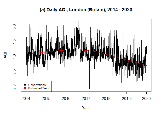
An optimal bandwidth of \(0.2422682\) was selected by the iterative
plug-in algorithm (IPI) within tsmoothlm(). A FARIMA (\(1, d, 0\)) was obtained from the
trend-adjusted residuals with \(\hat{d} =
0.1032687\) and \(\hat{\phi} =
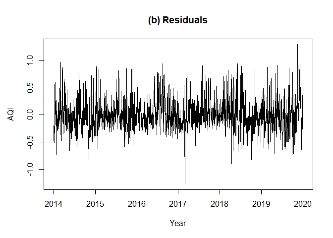
0.5435804\). Moreover, the estimated trend fits the data suitably
and the residuals seem to be stationary.
The trend estimation in combination with a fitted FARIMA model for the trend-adjusted values as in Example 1 is an ESEMIFAR model. With version 2.0.0 of the package, forecasting for based on such fitted ESEMIFAR models can be conducted using a designated predict-method. When applying that method, the user has the option between forecasting intervals based on the normality assumption for the innovations or based on a bootstrap.
h <- 200

# Via a bootstrap
set.seed(123)
fc <- predict(results, n.ahead = h, method = "boot")
head(fc$mean, 2)
#> [1] 4.135976 3.995659
head(fc$lower, 2)
#>           95%      99%
#> [1,] 3.725928 3.534129
#> [2,] 3.510523 3.330463
head(fc$upper, 2)
#>           95%      99%
#> [1,] 4.589879 4.749304
#> [2,] 4.531115 4.723409

# Under normality
fc <- predict(results, n.ahead = h, method = "norm")
head(fc$mean, 2)
#> [1] 4.135976 3.995659
head(fc$lower, 2)
#>           95%      99%
#> [1,] 3.717548 3.586068
#> [2,] 3.497323 3.340734
head(fc$upper, 2)
#>           95%      99%
#> [1,] 4.554404 4.685883
#> [2,] 4.493994 4.650583
Moreover, a quick plot of the results can be generated using a designated plot-method.
t_step <- diff(tail(t, 2))
t2 <- c(t, seq(from = tail(t, 1) + t_step, by = t_step, length.out = h))
plot(fc, t = t2, xlab = "Year", ylab = "AQI",
     main = "Point forecasts with 95%- and 99%-forecasting intervals")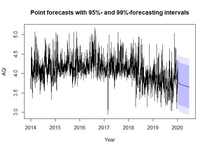
The trend estimation function can also be used for the implementation of semiparametric generalized autoregressive conditional heteroskedasticity (Semi-GARCH) models with long memory in Financial Econometrics (see Letmathe et al., 2023).
In esemifar three functions are available.
Original functions since version 1.0.0:
dsmoothlm: Data-driven Local Polynomial for the Trend’s
Derivatives in Equidistant Time SeriescritMatlm: FARIMA Order Selection Matrixtsmoothlm: Advanced Data-driven Nonparametric
Regression for the Trend in Equidistant Time SeriesOriginal functions since version 2.0.0:
predict.esemifar: ESEMIFAR Prediction Methodarma_to_ma: MA Representation of an ARMA Modelarma_to_ar: AR Representation of an ARMA Modeld_to_coef: Filter Coefficients of the Fractional
Differencing Operatorfarima_to_ma: MA Representation of a FARIMA Modelfarima_to_ar: AR Representation of a FARIMA ModelairLDN: Daily observations of individual air pollutants
from 2014 to 2020gdpG7: Quarterly G7 GDP between Q1 1962 and Q4
2019