| Type: | Package |
| Title: | Hierarchical Optimal Matching and Machine Learning Toolbox |
| Version: | 0.9.8 |
| Date: | 2025-12-08 |
| Author: | Teemu Daniel Laajala [aut, cre] |
| Maintainer: | Teemu Daniel Laajala <teelaa@utu.fi> |
| Depends: | R (≥ 3.0.0) |
| Imports: | grDevices, graphics, stats, utils |
| Suggests: | lme4, nlme, amap, nbpMatching, lattice, lmerTest, xtable, Cairo, Matrix, MASS |
| Description: | Various functions and algorithms are provided here for solving optimal matching tasks in the context of preclinical cancer studies. Further, various helper and plotting functions are provided for unsupervised and supervised machine learning as well as longitudinal mixed-effects modeling of tumor growth response patterns. |
| License: | GPL-2 | GPL-3 [expanded from: GPL (≥ 2)] |
| NeedsCompilation: | no |
| Packaged: | 2025-12-08 17:32:08 UTC; teemu |
| Repository: | CRAN |
| Date/Publication: | 2025-12-09 06:10:51 UTC |
Hierarchical Optimal Matching and Machine Learning Toolbox
Description
This package provides functions and algorithms for solving optimal matching tasks in the context of preclinical cancer studies. Further, various help and plotting functions are provided for unsupervised and supervised machine learning as well as longitudinal modeling of tumor growth response patterns.
Author(s)
Teemu Daniel Laajala
Maintainer: Teemu Daniel Laajala <teelaa@utu.fi>
References
Laajala TD, Jumppanen M, Huhtaniemi R, Fey V, Kaur A, et al. (2016) Optimized design and analysis of preclinical intervention studies in vivo. Sci Rep. 2016 Aug 2;6:30723. doi: 10.1038/srep30723.
Knuuttila M, Yatkin E, Kallio J, Savolainen S, Laajala TD, et al. (2014) Castration induces upregulation of intratumoral androgen biosynthesis and androgen receptor expression in orthotopic VCaP human prostate cancer xenograft model. Am J Pathol. 2014 Aug;184(8):2163-73. doi: 10.1016/j.ajpath.2014.04.010.
Examples
##
## Exploring the VCaP dataset provided alongside the 'hamlet' package
##

data(vcapwide)
data(vcaplong)

# VCaP Castration-resistant prostate cancer (CRPC) PSA-measurements (and body weight) in wide-format
mixplot(vcapwide[,c("PSAWeek10", "PSAWeek14", "BWWeek10", "Group")], pch=16)
anv <- aov(PSA ~ Group, data.frame(PSA = vcapwide[,"PSAWeek14"], Group = vcapwide[,"Group"]))
summary(anv)
TukeyHSD(anv)
summary(aov(BW ~ Group, data.frame(BW = vcapwide[,"BWWeek14"], Group = vcapwide[,"Group"])))

# VCaP Castration-resistant prostate cancer (CRPC) PSA-measurements (and body weight) in long-format
library(lattice)
xyplot(log2PSA ~ DrugWeek | Group, data = vcaplong, type="l", group=ID, layout=c(3,1))
xyplot(BW ~ DrugWeek | Group, data = vcaplong, type="l", group=ID, layout=c(3,1))

##
## Example multigroup (g=3) nbp-matching using the branch and bound algorithm,
## and subsequent random allocation of submatches to 3 arms
##

# Construct an Euclidean distance example distance matrix using 15 observations from the VCaP study
d <- as.matrix(dist(vcapwide[1:15,c("PSAWeek10", "BWWeek10")]))
# Matching using the b&b algorithm to submatches of size 3
# (which will result in 3 intervention groups)
bb3 <- match.bb(d, g=3)
str(bb3)

solvec <- bb3$solution
# matching vector, where each element indicates to which submatch each observation belongs to

# Perform an example random allocation of the above submatches,
# these will be randomly allocated to 3 arms based on the submatches
set.seed(1)
groups <- match.allocate(solvec)

# Illustrate randomization, no baseline differences in these three artificial groups
by(vcapwide[1:15,c("PSAWeek10", "BWWeek10")], INDICES=groups, FUN=function(x) x)

summary(aov(PSAWeek10 ~ groups, data = data.frame(PSAWeek10 = vcapwide[1:15,"PSAWeek10"], groups)))
summary(aov(BWWeek10 ~ groups, data = data.frame(BWWeek10 = vcapwide[1:15,"BWWeek10"], groups)))

##
## Example mixed-effects modeling of the longitudinal PSA profiles using
## the actual experimental groups
##

exdat <- vcaplong[vcaplong[,"Group"] %in% c("Vehicle", "ARN"),]

library(lme4)
# Model fitting using lme4-package
f1 <- lmer(log2PSA ~ 1 + DrugWeek + DrugWeek:ARN + (1 + DrugWeek|ID), data = exdat)

mem.getcomp(f1)

library(lmerTest)
# Model term testing using the lmerTest-package
summary(f1)
Extend range of variable limits while retaining a point of symmetricity
Description
This function serves as an alternative to the R function 'extendrange', when user wishes to conserve a point of symmetricity for the range. For example, this might be desired when the plot should be symmetric around the origin x=0, but that the sides need to extend beyond the actual range of values.
Usage
extendsymrange(x, r = range(x, na.rm = T), f = 0.05, sym = 0)
Arguments
x |
Vector of values to compute the range for |
r |
The range of values |
f |
The factor by which the range is extended beyond the extremes |
sym |
The defined point of symmetricity |
Value
A vector of 2 values for the lower and higher limit of the symmetric extended range
Author(s)
Teemu Daniel Laajala <teelaa@utu.fi>
See Also
Examples
set.seed(1)
ex <- rnorm(10)+2

hist(ex, xlim=extendsymrange(ex, sym=0), breaks=100)
Plot-region based heatmap
Description
This function plots heatmap figure based on the normal plot-region. This is useful if the image-based function 'heatmap' is not suitable, i.e. when multiple heatmaps should be placed in a single device.
Usage
hmap(x,
	add = FALSE,
	xlim = c(0.2, 0.8),
	ylim = c(0.2, 0.8),
	col = heat.colors(10),
	border = matrix(NA, nrow = nrow(x), ncol = ncol(x)),
	lty = matrix("solid", nrow = nrow(x), ncol = ncol(x)),
	lwd = matrix(1, nrow = nrow(x), ncol = ncol(x)),
	hclustfun = hclust,
	distfun = dist,
	reorderfun = function(d, w) reorder(d, w),
	textfun = function(xseq, yseq, labels, type = "row", ...)
		{ if (type == "col") par(srt = 90);
		text(x = xseq, y = yseq, labels = labels, ...);
		if (type == "col") par(srt = 0)},
	symm = F,
	Rowv = NULL,
	Colv = if (symm) Rowv else NULL,
	leftlim = c(0, 0.2), toplim = c(0.8, 1),
	rightlim = c(0.8, 1), bottomlim = c(0, 0.2),
	type = "rect",
	scale = c("none", "row", "column"),
	na.rm = T,
	nbins = length(col),
	valseq =
		seq(from = min(x, na.rm = na.rm),
		to = max(x, na.rm = na.rm), length.out = nbins),
	namerows = TRUE,
	namecols = TRUE,
	...)
Arguments
x |
Matrix to be plotted |
add |
Should the figure be added to the plotting region of an already existing figure |
xlim |
The x limits in which the heatmap is placed horizontally in the plotting region |
ylim |
The y limits in which the heatmap is placed vertically in the plotting region |
col |
Color palette for the heatmap colors |
border |
A matrix of border color definitions (rectangles in the heatmap) |
lty |
A matrix of line type definitions (rectangles in the heatmap) |
lwd |
A matrix of line width definitions (rectangles in the heatmap) |
hclustfun |
The hierarchical clustering function similar to 'stats::heatmap' implementation. Should yield a valid 'hclust' object for a given distance/dissimilarity matrix. |
distfun |
The distance/dissimilarity function similar to 'stats::heatmap' implementation. Should yield a valid 'dist' object for a given data matrix. |
reorderfun |
The function to use to reorder branches of the clustering (notice that same-level branches in a hierarchical clustering may be permutated without violating the solution). The default approach from 'stats::heatmap' is utilized here. |
textfun |
A text function that is used to plot the names of the rows and columns, if desired. The default implementation shows how user could tailor the columns and rows differently, by turning the column labels around 90-degrees. The parameter 'type' is used to distinguish between rows and columns. |
symm |
Should the given data matrix be treated as symmetric (has to be a square matrix if so), by default 'FALSE'. |
Rowv |
The row clustering parameter. If 'NA' the row hierarchical clustering is completely omitted. Alternatively, if a numeric vector of ranks, the ordering of branches is tried to be permutated according to the desired order. This can also be a pre-computed dendrogram-object. |
Colv |
The column clustering parameter. If 'NA' the column hierarchical clustering is completely omitted. Alternatively, if a numeric vector of ranks, the ordering of branches is tried to be permutated according to the desired order. This can also be a pre-computed dendrogram-object. |
leftlim |
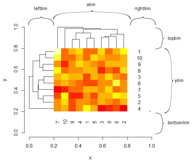
The horizontal limits of the row hierarchical clustering. The horizontal limits of the heatmap are {a=leftlim[1], b=leftlim[2], c=xlim[1], d=xlim[2]} where the 'a' is where the row dendrogram begins, 'b' is where the row dendrogram ends, 'c' is where the heatmap itself begins, and 'd' is where the heatmap itself ends. The vertical limits are computed according to 'ylim' to align correctly with the heatmap rectangles. |
toplim |
The vertical limits of the row hierarchical clustering. The horizontal limits of the heatmap are {a=ylim[1], b=ylim[2], c=toplim[1], d=toplim[2]} where the 'a' is where the heatmap begins, 'b' is where the heatmap ends, 'c' is where the column dendrogram begins, and 'd' is where the column dendrogram ends. The horizontal limits are computed according to 'xlim' to align correctly with the heatmap rectangles. |
rightlim |
The horizontal limits for the row texts. |
bottomlim |
The vertical limits for the column texts. |
type |
Type of clustering visualization; while default "rect" provides a rectangular-angled tree, the alternate option "tri" provides triangular-angled tree. |
scale |
Should data be scaled according to 'row' or 'column' (or 'col') similarly to 'stats::heatmap'. |
na.rm |
Should missing values be removed, by default TRUE. |
nbins |
Number of discrete bins the data is divided into using 'seq(from=min(x), to=max(x), length.out=nbins)'. |
valseq |
The sequence of values by which the data is binned, typically corresponding to the above 'nbins' parameter. |
namerows |
If a single boolean value TRUE, then the default 'rownames(x)' are plotted to the right of the rows with the 'textfun'. If it is a vector of length 'nrow(x)', then this vector is used for plotting the row names instead. |
namecols |
If a single boolean value TRUE, then the default 'colnames(x)' are plotted below the columns with the 'textfun'. If it is a vector of length 'nrow(x)', then this vector is used for plotting the column names instead. |
... |
Additional parameters provided to the rectangle plotting function |
Author(s)
Teemu Daniel Laajala <teelaa@utu.fi>
See Also
heatmap
hmap.key
hmap.annotate
Examples
# Generate some data
set.seed(1)
r1 <- replicate(30, rnorm(20))
lab <- sample(letters[1:2], 20, replace=TRUE)
r1[lab==lab[1],] <- r1[lab==lab[1],] + 2
r2a <- replicate(10, rnorm(10))
r2b <- replicate(10, rnorm(10))

# Set up a new plot region, notice we have a 2-fold wider x-axis
plot.new()
plot.window(xlim=c(0,2), ylim=c(0,1))

# Plot an example plot along with the color key and annotations for our 'lab' vector
h1 <- hmap(r1, add = TRUE)
hmap.key(h1, x1=0.18)
hmap.annotate(h1, rw = lab, rw.wid=c(0.82,0.90))

# Plot the rest to show how the coordinates are adjusted to place the heatmap(s) differently
h2a <- hmap(r2a, add = TRUE, xlim=c(1.2, 1.8), leftlim=c(1.0, 1.2),
	rightlim=c(1.8,2.0), ylim=c(0.6, 1.0), bottomlim=c(0.5,0.6), Colv=NA)
h2b <- hmap(r2b, add = TRUE, xlim=c(1.2, 1.8), leftlim=c(1.0, 1.2),
	rightlim=c(1.8,2.0), ylim=c(0.1, 0.5), bottomlim=c(0.0,0.1), Colv=NA)

# Show the normal plot region axes
axis(1, at=c(0.5,1.5), c("A", "B"))

## Not run:
	# Heatmap used as base for the help documentation figure
	set.seed(1)
	hmap(matrix(rnorm(100), nrow=10), xlim=c(0.2,0.8), ylim=c(0.2,0.8),
		leftlim=c(0.0,0.2), rightlim=c(0.8,1.0),
		bottomlim=c(0.0,0.2), toplim=c(0.8,1.0))
	axis(1); axis(2); title(xlab="x", ylab="y")

## End(Not run)
Add a row and column annotations to a plot-region based heatmap built with 'hmap'
Description
Annotation of rows or columns in a 'hmap'-plot. By default, rectangles aligned with either rows or columns are plotted to the right-side or lower-side of the heatmap respectively. User-specified customizations may be given to change these annotations in positioning or type.
Usage
hmap.annotate(h, rw, rw.n = length(unique(rw)), rw.col = rainbow(rw.n,
                 start = 0.05, end = 0.5), rw.wid, rw.hei, rw.pch,
                 rw.x = rep(min(h$rightlim), times =
                 length(h$rowtext$xseq)), rw.y = h$rowtext$yseq, rw.shift
                 = c(0.02, 0), cl, cl.n
                 = length(unique(cl)), cl.col = rainbow(cl.n, start =
                 0.55, end = 1), cl.wid, cl.hei, cl.pch, cl.x =
                 h$coltext$xseq, cl.y = rep(max(h$bottomlim), times =
                 length(h$coltext$yseq)), cl.shift = c(0, -0.02), ...)
Arguments
h |
The list of heatmap parameters returned invisibly by the original 'hmap'-call. |
rw |
Annotation vector for rows 'r', each unique instance is given a different color (or pch) and plotted right-side of the corresponding heatmap rows |
rw.n |
Number of unique colors (or pch) to give each annotated row |
rw.col |
A vector for color values for unique instances in 'r' for annotating rows |
rw.wid |
The widths for annotation boxes for each row 'r' |
rw.hei |
The heights for annotation boxes for each row 'r' |
rw.pch |
Alternatively, instead of widths and heights user may specify a symbol 'pch' to use for annotating each row |
rw.x |
The x-coordinate locations for the row annotations, by default right side of heatmap itself |
rw.y |
The y-coordinate locations for the row annotations, by default same vertical locations as for the heatmap rows |
rw.shift |
Row annotation shift: a vector of 2 values, where first indicates the amount of x-axis shift desired and the second indicates the amount of y-axis shift |
cl |
Annotation vector for columns 'r', each unique instance is given a different color (or pch) and plotted lower-side of the corresponding heatmap columns |
cl.n |
Number of unique colors (or pch) to give each annotated column |
cl.col |
A vector for color values for unique instances in 'c' for annotating columns |
cl.wid |
The widths for annotation boxes for each column 'c' |
cl.hei |
The heights for annotation boxes for each column 'c' |
cl.pch |
Alternatively, instead of widths and heights user may specify a symbol 'pch' to use for annotating each column |
cl.x |
The x-coordinate locations for the column annotations, by default same horizontal locations as for the heatmap columns |
cl.y |
The y-coordinate locations for the column annotations, by default lower side of heatmap itself |
cl.shift |
Column annotation shift: a vector of 2 values, where first indicates the amount of x-axis shift desired and the second indicates the amount of y-axis shift |
... |
Additional parameters supplied either to 'rect' or 'points' function if user desired rectangles or 'pch'-based points respectively |
Author(s)
Teemu Daniel Laajala <teelaa@utu.fi>
See Also
Examples
# Generate some data
set.seed(1)
r1 <- replicate(30, rnorm(20))
lab <- sample(letters[1:2], 20, replace=TRUE)
r1[lab==lab[1],] <- r1[lab==lab[1],] + 2
r2a <- replicate(10, rnorm(10))
r2b <- replicate(10, rnorm(10))

# Set up a new plot region, notice we have a 2-fold wider x-axis
plot.new()
plot.window(xlim=c(0,2), ylim=c(0,1))

# Plot an example plot along with the color key and annotations for our 'lab' vector
h1 <- hmap(r1, add = TRUE)
hmap.key(h1, x1=0.18)
hmap.annotate(h1, rw = lab, rw.wid=c(0.82,0.90))

# Plot the rest to show how the coordinates are adjusted to place the heatmap(s) differently
h2a <- hmap(r2a, add = TRUE, xlim=c(1.2, 1.8), leftlim=c(1.0, 1.2),
	rightlim=c(1.8,2.0), ylim=c(0.6, 1.0), bottomlim=c(0.5,0.6), Colv=NA)
h2b <- hmap(r2b, add = TRUE, xlim=c(1.2, 1.8), leftlim=c(1.0, 1.2),
	rightlim=c(1.8,2.0), ylim=c(0.1, 0.5), bottomlim=c(0.0,0.1), Colv=NA)

# Show the normal plot region axes
axis(1, at=c(0.5,1.5), c("A", "B"))
Add a color key to a plot-region based heatmap built with 'hmap'
Description
A continuous color scale key for a heatmap. By default the key is constructed according to the 'h'-object which is invisibly returned by the original 'hmap'-call. Some customization may be supplied to position the legend or to customize ticks and style.
Usage
hmap.key(h, x0 = h$leftlim[1], x1 = h$leftlim[2], y0 =
                 h$toplim[1], y1 = h$toplim[2], xlim = range(h$valseq),
                 ratio = 0.5, tick = 0.1, at = seq(from =
                 min(h$valseq), to = max(h$valseq), length.out = 5),
                 bty = "c", cex = 0.5, pos = 3, offset = c(0,0))
Arguments
h |
The list of heatmap parameters returned invisibly by the original 'hmap'-call. |
x0 |
Coordinates for the color key; left border |
x1 |
Coordinates for the color key; right border |
y0 |
Coordinates for the color key; lower border |
y1 |
Coordinates for the color key; upper border |
xlim |
Value range for the x-axis within the key itself, by default extracted from the h-object |
ratio |
Ratio between y-axis coordinates to separate the key box to upper color key box and lower tick and values |
tick |
The vertical length in value ticks |
at |
The values in color key at which to plot ticks and the values at ticks |
bty |
Type of box to plot around the color key |
cex |
The zooming factor for plotting the text and other objects affected by the 'cex' parameter in 'par' |
pos |
The text alignment and position parameter given to the 'text' function in the key |
offset |
Allows offsetting legend text by absolute {x,y} coordinates in relation to ticks |
Author(s)
Teemu Daniel Laajala <teelaa@utu.fi>
See Also
Examples
# Generate some data
set.seed(1)
r1 <- replicate(30, rnorm(20))
lab <- sample(letters[1:2], 20, replace=TRUE)
r1[lab==lab[1],] <- r1[lab==lab[1],] + 2
r2a <- replicate(10, rnorm(10))
r2b <- replicate(10, rnorm(10))

# Set up a new plot region, notice we have a 2-fold wider x-axis
plot.new()
plot.window(xlim=c(0,2), ylim=c(0,1))

# Plot an example plot along with the color key and annotations for our 'lab' vector
h1 <- hmap(r1, add = TRUE)
hmap.key(h1, x1=0.18)
hmap.annotate(h1, rw = lab, rw.wid=c(0.82,0.90))

# Plot the rest to show how the coordinates are adjusted to place the heatmap(s) differently
h2a <- hmap(r2a, add = TRUE, xlim=c(1.2, 1.8), leftlim=c(1.0, 1.2),
	rightlim=c(1.8,2.0), ylim=c(0.6, 1.0), bottomlim=c(0.5,0.6), Colv=NA)
h2b <- hmap(r2b, add = TRUE, xlim=c(1.2, 1.8), leftlim=c(1.0, 1.2),
	rightlim=c(1.8,2.0), ylim=c(0.1, 0.5), bottomlim=c(0.0,0.1), Colv=NA)

# Show the normal plot region axes
axis(1, at=c(0.5,1.5), c("A", "B"))
Allocation of matched units to intervention arms
Description
This function allocates units belonging to a single submatch to separate intervention arms. This ensures that the resulting intervention groups are homogeneous in respect to the variables that were used to construct the distance/dissimilarity matrix for the non-bipartite matching. The number of resulting intervention groups is equal to the 'g' (i.e. submatch size) used in the multigroup non-bipartite matching.
Usage
match.allocate(xmat)
Arguments
xmat |
A binary matching matrix or a matching vector given by match.bb-function. |
Value
A vector where each element indicates to which group the observation was randomized to. The group names are "Group_A", "Group_B", "Group_C", ... until 'g' letters, where 'g' was the size of submatches.
Author(s)
Teemu Daniel Laajala <teelaa@utu.fi>
See Also
match.bb
match.mat2vec
match.vec2mat
match.dummy
Examples
data(vcapwide)

# Construct an Euclidean distance example distance matrix using 15 observations from the VCaP study
d <- as.matrix(dist(vcapwide[1:15,c("PSAWeek10", "BWWeek10")]))
# Matching using the b&b algorithm to submatches of size 3
# (which will result in 3 intervention groups)
bb3 <- match.bb(d, g=3)
str(bb3)

solvec <- bb3$solution
# matching vector, where each element indicates to which submatch each observation belongs to

# Perform an example random allocation of the above submatches,
# these will be randomly allocated to 3 arms based on the submatches
set.seed(1)
groups <- match.allocate(solvec)

# Illustrate randomization, no baseline differences in these three artificial groups
by(vcapwide[1:15,c("PSAWeek10", "BWWeek10")], INDICES=groups, FUN=function(x) x)

summary(aov(PSAWeek10 ~ groups, data = data.frame(PSAWeek10 = vcapwide[1:15,"PSAWeek10"], groups)))
summary(aov(BWWeek10 ~ groups, data = data.frame(BWWeek10 = vcapwide[1:15,"BWWeek10"], groups)))
Branch and Bound algorithm implementation for performing multigroup non-bipartite matching
Description
This function performs multigroup non-bipartite matching of observations based on a provided distance/dissimilarity matrix 'd'. The number of elements in each submatch is defined by the parameter 'g'.
Usage
match.bb(d, g = 2, presort = "complete", progress = 1e+05,
bestknown = Inf, maxbranches = Inf, verb = 0)
Arguments
d |
A distance matrix with NxN elements |
g |
Number of elements per each submatch, i.e. how many observations are always matched together |
presort |
If hierarchical clustering should be used for an initial guess, hclust method-options are valid options ("complete", "single", "ward", "average") |
progress |
How many branching operations are done before outputting information to the user |
bestknown |
If a best known solution already exists, this can be used to bound branches of the tree before initiation. The default Inf value causes whole search tree to be potential solution space. |
maxbranches |
Maximum number of branching operations before returning current best solution, by default no cutoff is defined. |
verb |
Level of verbosity |
Details
See further details in the reference Laajala et al.
Value
The function returns a list of objects, where elements are
branches |
Number of branching operations during the branch and bound algorithm |
bounds |
Number of bounding operations during the branch and bound algorithm |
ends |
Number of end leaf nodes visited during the branch and bound algorithm |
matrix |
The resulting binary matching matrix where rows and columns sum to g |
solution |
The resulting matching vector where each element indicates the submatch where the observation was placed |
cost |
Final cost value of the target function in the minimization task |
Note
Notice that the solution submatch vector in $solution is not the same as the intervention group allocation. Submatches should be randomly allocated to intervention arms using the match.allocate-function.
The package 'nbpMatching' provides a FORTRAN implementation for computation of paired non-bipartite matching case (g=2).
Computation may be heavy if the number of observations is high, or the number of within-submatch pairwise distances to consider is high (increases quadratically as a function of 'g').
Author(s)
Teemu Daniel Laajala <teelaa@utu.fi>
See Also
match.allocate
match.mat2vec
match.vec2mat
match.dummy
Examples
data(vcapwide)

# Construct an Euclidean distance example distance matrix using 15 observations from the VCaP study
d <- as.matrix(dist(vcapwide[1:15,c("PSAWeek10", "BWWeek10")]))

bb3 <- match.bb(d, g=3)
str(bb3)

mat <- bb3$matrix
# binary matching matrix
solvec <- bb3$solution
# matching vector, where each element indicates to which submatch each observation belongs to

mixplot(data.frame(vcapwide[1:15,c("PSAWeek10", "BWWeek10")],
 submatch=as.factor(paste("Submatch_",solvec, sep=""))), pch=16, col=rainbow(5))
Create dummy individuals or sinks to a data matrix or a distance/dissimilarity matrix
Description
Dummy observations are allowed in order to make the number of observations dividable by the number of elements in each submatch, i.e. for pairwise matching the number of observations should be paired, for triangular matching the number of observations should be dividable by 3, etc. This can be done either by adding column averaged individuals to the original data frame (parameter 'dat'), or by adding zero distance sinks to the distance/dissimilarity matrix (parameter 'd'). The latter approach favors dummies being matched to real extreme observations, while the former favors dummies being matched to close-to-mean real observations.
Usage
match.dummy(dat, d, g = 2)
Arguments
dat |
A data.frame of the original observations, to which column averaged new dummy observations are added |
d |
N times N distance/dissimilarity matrix, to which zero distance sinks are added |
g |
The desired number of elements per each submatch, i.e. the size of the clusters. The number of added dummies is the smallest number of additions that fulfills (N+dummy)%%g == 0 |
Value
Depending on if the dat or the d parameter was provided, the function either: dat: adds new averaged individuals according to column means and then returns the data matrix d: adds zero distance sinks to the distance/dissimilarity matrix and returns the new distance/dissimilarity matrix
Note
Adding zero distance sinks to the distance matrix or averaged individuals to the original data frame produce different results and affect the optimal matching task differently.
Author(s)
Teemu Daniel Laajala <teelaa@utu.fi>
See Also
match.allocate
match.mat2vec
match.vec2mat
match.bb
Examples
data(vcapwide)

exdat <- vcapwide[1:10,c("PSAWeek10", "BWWeek10")]
dim(exdat)
avgdummies <- match.dummy(dat=exdat, g=3)
dim(avgdummies)
# Construct an Euclidean distance matrix after adding two dummy individuals
# (averaged individuals to the original data matrix)
bb3 <- match.bb(as.matrix(dist(avgdummies)), g=3)
str(bb3)

# Construct an Euclidean distance matrix after adding two dummy distances (zero distance sinks)
exd <- as.matrix(dist(vcapwide[1:10,c("PSAWeek10", "BWWeek10")]))
dim(exd)
d <- match.dummy(d=exd, g=3)
dim(d)
# 10 is not dividable by 3, 2 sinks are added to make d 12x12
bb3 <- match.bb(d, g=3)
str(bb3)

# Notice that sinks produce a lot smaller target function costs than averaged individuals
Non-bipartite matching using the Genetic Algorithm (GA)
Description
An implementation of the Genetic Algorithm for solving non-bipartite matching tasks with customizable evolutionary events and parameters
Usage
match.ga(d, g,
	pops,
	generations = 100,
	popsize = 100,
	nmutate = 100,
	ndeath = 30,
	type = "min",
	mutate = .ga.mutate,
	breed = .ga.breed,
	weight = .ga.weight,
	fitness = .ga.fitness,
	step = .ga.step,
	initialize = .ga.init,
	progplot = TRUE,
	plot = TRUE,
	verb = 0,
	progress = 500,
	...)
Arguments
d |
A distance/dissimilarity matrix 'd' |
g |
The size in submatches, as in how many observations are always connected |
pops |
If user wants to specify starting populations, they can be provided here as a matrix. Each row correspondings to the observations, while columns are the different solutions (population in the GA). For example, a 10 row 100 column pops-matrix would be 100 different matching solutions of 10 observations. Each number in the matrix indicates a different submatch. |
generations |
Number of simulations to run in the GA. In each step, mutations, breeding and breeding occur according to user's specified settings, and a new generation is created out of this. |
popsize |
Number of solutions (='individuals') to have in each step of the algorithm. |
nmutate |
Number of mutations to occur in each step. Individuals are sampled with replacement, and then given the corresponding number of mutations. |
ndeath |
Number of deaths to occur in each step. Each dead solution (='individual') is then replaced by breeding suitable parents (probability of being a parent weighted by fitness). |
type |
Type of optimization, can be 'min' or 'max'. |
mutate |
Mutation function; by default the hamlet internal function '.ga.mutate' is used. This function takes in solution vector 'x'. Two random positions are then swapped, which could be seen as a form of a point mutation. |
breed |
Breeding function; by default the hamlet internal function '.ga.breed' is used. This function takes in solution vectors 'x' and 'y' ,which will be the parents, and the distance matrix 'd'. The products x*d and y*d are computed, and row-wise differences are computed between the two matrices. The row with the highest difference indicates where one of the parents can be most improved, and this trait is inherited from the other parent. |
weight |
Weighting function; by default the hamlet internal function '.ga.weight' is used. This weight should be correspond to probabilities that the corresponding individuals will undergo some sort of event (i.e. mutation, death) or participate in producing offspring (i.e. breed). This probability weight is computed according to ranks of fitnesses computed in the |
fitness |
Fitness function; by default the hamlet internal function '.ga.fitness' is used. This should yield the numeric fitness for a solution, indicating how viable the solution is in relation to the others. In a minimization task the lower fitness indicates better viability. |
step |
A step function; by default the hamlet internal function '.ga.step' is used. The step function which combines all operations in the GA, in order to produce the next generation of solutions given the previous one. |
initialize |
Initialization function; by default the hamlet internal function '.ga.initialize' is used. This function should format a set of valid solutions to produce the first generation in the beginning of the GA. |
progplot |
Should progress be plotted. If true, in every generation index dividable by the parameter 'progress', a function of fitnesses over the generations is plotted. The plot shows development of solution cost quantiles over time. |
plot |
Should the function plot the final quantiles over all the generations. |
verb |
Level of verbosity; -1 indicates omitting of verbal output, 0 indicates normal level, and +1 indicates debugging/additional information. |
progress |
How often should the function plot and print intermediate information on the progress. |
... |
Additional parameters for the internal GA functions. |
Details
The Genetic Algorithm (GA) is a form of an evolutionary optimization algorithm, where a population (a group of solutions to an optimization tasks) reproduce among themselves, die, mutate, and live on in a simulated environment. As the GA is a generic framework of solution approaches, it has many adjustable parameters and user may wish to explore many different options for the populations (for example in population size, mutation frequencies, fitness functions, drift etc) and also the evolutionary mechanics (such as breeding technique, types of mutations, and suitability for reproducing). Here, general default options and mechanics are provided, but it is advisable to explore different parameters for the particular optimization task in hand to find optimal solutions. If the user wishes to explore the implementation of the default mechanics, the function implementations are internally available in the hamlet-package. For example, the mutation function is accessible with the command: ' hamlet::.ga.mutate '.
Value
The returned list compromises of:
A list of solutions; a matrix 'pops' which contains the population of solutions in the final generation of the algorithm, a vector 'fitnesses' which portrait the corresponding fitnesses to the columns of 'pops', and 'weights' which were the corresponding probabilities to events in the GA.
A vector 'bestsol', for which the fitness function obtained minimum (or maximum) value during the algorithm.
A value 'best', which is the optimum solution cost value observed during the algorithm.
Note
Notice that end quality of the matching based allocation is heavily dependent on providing a feasible matrix D. One should carefully consider choice and tuning of the similarity metric. For example, Euclidean distance without standardization is often not a good choice as it does not normalize the variance of each variable and emphasis is on baseline variables that have a large relative variance.
Note that the R-package 'GA' offers a wide range of generalized GA-related tools.
Author(s)
Teemu Daniel Laajala <teelaa@utu.fi>
See Also
Examples
# Set up a distance matrix and add dummies, then run GA
data(vcapwide)

# Construct an Euclidean distance example distance matrix using 15 observations from the VCaP study
d <- as.matrix(dist(vcapwide[1:15,c("PSAWeek10", "BWWeek10")]))
# Or rather, z-score transform all input variables first
d2 <- as.matrix(dist(scale(vcapwide[1:15,c("PSAWeek10", "BWWeek10")])))

# Notice that random simulations take place, so we will fix the RNG seed for reproducibility
set.seed(1)
# Resulting genetic algorithm progression is plotted by default
ga <- match.ga(d2, g=3, generations=60)
str(ga)
# Submatches, i.e. similar individuals that ought to be allocated to separate groups
ga[[2]]
Transform a binary matching matrix to a matching vector
Description
This function transforms a binary matching matrix to a matching vector. A matching vector is of length N where each element indicates the submatch to which the observation belongs to. Notice that this is not the same as the group allocation vector that is provided by the match.allocate-function. The binary matching matrix is of size N x N where 0 indicates that the observations have been part of a different submatch, and 1 indicates that the observations have been part of the same submatch. Diagonal is always 0 although an observation is always in the same submatch with its self.
Usage
match.mat2vec(xmat)
Arguments
xmat |
A binary matching matrix 'xmat' |
Value
A matching vector where each element indicates submatch the observation belongs to
Note
Notice that the particular index numbers produced by match.mat2vec may be different to that of the branch and bound solution vector, but that the submatches shared by observations are common.
Author(s)
Teemu Daniel Laajala <teelaa@utu.fi>
See Also
match.allocate
match.bb
match.vec2mat
match.dummy
Examples
data(vcapwide)

# Construct an Euclidean distance example distance matrix using 15 observations from the VCaP study
d <- as.matrix(dist(vcapwide[1:15,c("PSAWeek10", "BWWeek10")]))

bb3 <- match.bb(d, g=3)
str(bb3)

mat <- bb3$matrix
# matching vector, where each element indicates to which submatch each observation belongs to

mat
solvec <- match.mat2vec(mat)
which(mat[1,] == 1)
# E.g. the first, third and thirteenth observation are part of the same submatch
which(solvec == solvec[1])
# Similarly
Transform a matching vector to a binary matching matrix
Description
This function allows transforming a matching vector to a binary matching matrix. A matching vector is of length N where each element indicates the submatch to which the observation belongs to. Notice that this is not the same as the group allocation vector that is provided by the match.allocate-function. The binary matching matrix is of size N x N where 0 indicates that the observations have been part of a different submatch, and 1 indicates that the observations have been part of the same submatch. Diagonal is always 0 although an observation is always in the same submatch with its self.
Usage
match.vec2mat(x)
Arguments
x |
A matching vector 'x' |
Value
N times N binary matching matrix, where 0 indicates that the observations have been part of a different submatch, and 1 indicates that the observations have been part of the same submatch.
Author(s)
Teemu Daniel Laajala <teelaa@utu.fi>
See Also
match.allocate
match.mat2vec
match.bb
match.dummy
Examples
data(vcapwide)

# Construct an Euclidean distance example distance matrix using 15 observations from the VCaP study
d <- as.matrix(dist(vcapwide[1:15,c("PSAWeek10", "BWWeek10")]))

bb3 <- match.bb(d, g=3)
str(bb3)

solvec <- bb3$solution
# matching vector, where each element indicates to which submatch each observation belongs to

solvec
mat <- match.vec2mat(solvec)
mat
which(mat[1,] == 1)
# E.g. the first, third and thirteenth observation are part of the same submatch
which(solvec == solvec[1])
# Similarly
Extract per-observation components for fixed and random effects of a mixed-effects model
Description
Assuming a mixed-effects model of form y_fit = Xb + Zu + e, where X is the model matrix for fixed effects, Z is the model matrix for random effects, and b and u are the fixed and random effects respectively, this function returns these components per each fitted value y. These may be useful for model inference and/or diagnostic purposes.
Usage
mem.getcomp(fit)
Arguments
fit |
A fitted mixed-effects model generated either through the lme4 or the nlme package. |
Details
Notice that per-observation model error is e = Xb + Zu - y_observation. Similarly, the components Xb and Zu are extracted.
Value
The function returns per-observation model fit components for a mixed-effects model. The return fields are
Xb |
Fixed effects component Xb |
Zu |
Random effects component Zu |
XbZu |
Full model fit by summing the above two Xb+Zu |
e |
Model error e |
y |
Original observations y |
Author(s)
Teemu Daniel Laajala <teelaa@utu.fi>
See Also
Examples
data(vcaplong)

exdat <- vcaplong[vcaplong[,"Group"] %in% c("Vehicle", "ARN"),]

library(lme4)
f1 <- lmer(log2PSA ~ 1 + DrugWeek + DrugWeek:ARN + (1 + DrugWeek|ID), data = exdat)

mem.getcomp(f1)
Plot random effects histograms for a fitted mixed-effects model
Description
This plot creates histogram plots for the columns extracted from random effects from a model fit. This is useful for model diagnostics, such as observing deviations from normality in the random effects.
Usage
mem.plotran(fit, breaks = 100)
Arguments
fit |
A fitted mixed-effects model generated either through the lme4 or the nlme package. |
breaks |
Number of breaks in the histograms (passed to the 'hist'-function) |
Author(s)
Teemu Daniel Laajala <teelaa@utu.fi>
See Also
Examples
data(vcaplong)

exdat <- vcaplong[vcaplong[,"Group"] %in% c("Vehicle", "ARN"),]

library(lme4)
f1 <- lmer(log2PSA ~ 1 + DrugWeek + DrugWeek:ARN + (1 + DrugWeek|ID), data = exdat)

ranef(f1) # Histograms are plotted for these columns
mem.plotran(f1)
Plot residuals of a mixed-effects model along with trend lines
Description
This function plots stylized residuals of a mixed-effects model. It is possible to obtain fitted values versus errors (XbZu vs e), or original values versus errors (y vs e) in order to obtain different views to the errors in connection to the observations.
Usage
mem.plotresid(fit, linear = T, type = "XbZu", main, xlab, ylab)
Arguments
fit |
A fitted mixed-effects model generated either through the lme4 or the nlme package. |
linear |
Should linear trend lines be drawn to the residual plot |
type |
Type of residual plot; should fitted values (value "XbZu") or original observations (value "y") be plotted against "e" errors |
main |
Main title |
xlab |
x-axis label |
ylab |
y-axis label |
Details
Notice that the typical residual plot is fitted values (type="XbZu") versus errors ("e").
Author(s)
Teemu Daniel Laajala <teelaa@utu.fi>
See Also
Examples
data(vcaplong)

exdat <- vcaplong[vcaplong[,"Group"] %in% c("Vehicle", "ARN"),]

library(lme4)
f0 <- lmer(log2PSA ~ 1 + DrugWeek + (1 + DrugWeek|ID), data = exdat)
f1 <- lmer(log2PSA ~ 1 + DrugWeek + DrugWeek:ARN + (1 + DrugWeek|ID), data = exdat)
f2 <- lmer(log2PSA ~ 1 + DrugWeek + DrugWeek:ARN + (1|ID) + (0 + DrugWeek|ID), data = exdat)
f3 <- lmer(log2PSA ~ 1 + DrugWeek + DrugWeek:ARN + (1|Submatch) + (0 + DrugWeek|ID), data = exdat)

par(mfrow=c(2,2))
mem.plotresid(f0)
mem.plotresid(f1)
mem.plotresid(f2)
mem.plotresid(f3)
Power simulations for the fixed effects of a mixed-effects model through structured bootstrapping of the data and re-fitting of the model
Description
Bootstrap sampling is used to investigate the statistical significance of the fixed effects terms specified for a readily fitted mixed-effects model as a function of the number of individuals participating in the study. User either specifies a suitable sampling unit, or it is automatically identified based on the random effects formulation of a readily fitted mixed-effects model. Per each count of individuals in vector N, a fixed number of bootstrapped datasets are generated and re-fitted using the model formulation on the pre-fitted model. Power is then computed as the fraction of effects identified as statistically significant out of all the bootstrapped datasets.
Usage
mem.powersimu(fit, N = 4:20, boot = 100, level = NULL, strata = NULL,
	default = FALSE, seed = NULL, plot = TRUE, plot.loess = FALSE,
	legendpos = "bottomright", return.data = FALSE, verb = 1, ...)
Arguments
fit |
A fitted mixed-effects model. Should be either a model produced by the lme4-package, or then a modified lme4-fit such as provided by lmerTest or similar package that builds on lme4. |
N |
A vector of desired amounts of individuals to be tested, i.e. sample sizes N. Notice that the N may be either a total N if no strata is spesified, or then an N value per each substrata if strata is not NULL. See below the parameter 'strata'. |
boot |
Number of bootstrapped datasets to generate per each N value. The total number of generated data frames in the end will be N times boot. |
level |
An unambiguous indicator available in the model data frame that indicates each separate individual unit in the experiment. For example, this may correspond to a single patient indicator column ID, where each patient has a unique ID instance. If this parameter is given as NULL, then this function automatically attempts to identify the best possible level of individual indicators based on the random effects specified for the model. |
strata |
If any sampling strata should be balanced, it should be indicated here. For example, if one is studying the possible effects of an intervention, it is typical to have an equal number of individual both in the control and in the intervention arms also in the sampled datasets. It should be then given as an column name available in the original model data frame. Each strata will be sampled in equal amounts. |
default |
What is the default statistical significance if a model could not be re-fitted to the sampled datasets, which may occur for example due to convergence or redundance issues. This defaults to FALSE, which means that a coefficient is expected to be statistically insignificant if the corresponding model re-fitting fails in lme4. |
seed |
For reproducibility, one may wish to set a numeric seed to produce the exact same results. |
plot |
If set to TRUE, the function will plot a power curve. Each fixed effects coefficient is a different curve, with color coding and a legend annotated to separate which one is which. |
plot.loess |
If plot==TRUE, this plot.loess==TRUE adds an additional loess-smoothed approximated curve to the existing curves. This is useful if running the simulations with a low number of bootstrapped samples, as it may help approximate where the curve reaches critical points, i.e. power = 0.8. |
legendpos |
Position for the legend in plot==TRUE, defaults to "bottomright". Any legal position similar to provided the function 'legend' is allowed. |
return.data |
Should one obtain the bootstrapped data instead of bootstrapping and then re-fitting. This will skip the model re-fitting schema and instead return a list of lists with the bootstrapped data instead. The outer list corresponds to the values of 'N', while the inner loop corresponds to the different 'boot' runs of bootstrap. This may be useful to inspecting that the schema is sampling correct sampling units for example, or if bootstrapping is to be used for something else than re-fitting the lme4-models. |
verb |
Numeric value indicating the level of verbosity; 0=silent, 1=normal, 2=debugging. |
... |
Additional parameters provided for the function. |
Details
This function will by default utilizes the lmerTest-package's Satterthwaite approximation for determining the p-values for the fixed effects. If this fails, it resorts to the conventional approximation |t|>2 for significance, which is not accurate, but may provide a reasonable approximation for the power levels.
Value
If return.data==FALSE, this function will return a matrix, where the rows correspond to the different N values and the columns correspond to the fixed effects. The values [0,1] are the fraction of bootstrapped datasets where the corresponding fixed effects was detected as statistically significant.
Note
Please note that the example runs in this document are extremely small due to run time constraints on CRAN. For real power analyses, it is recommended that the N counts would vary e.g. from 5 to 15 with steps of 1 and the amount of bootstrapped datasets would be at least 100.
Author(s)
Teemu D. Laajala
See Also
Examples
# Use the VCaP ARN data as an example
data(vcaplong)
arn <- vcaplong[vcaplong[,"Group"] == "Vehicle" | vcaplong[,"Group"] == "ARN",]

# lme4 is required for mixed-effects models
library(lme4)
# Fit an example fixed effects model
fit <- lmer(PSA ~ 1 + DrugWeek + ARN:DrugWeek + (1|ID) + (0 + DrugWeek|ID), data = arn)

# For reproducibility, set a seed
set.seed(123)
# Run a brief power analysis with only a few selected N values and a limited number of bootstrapping
# Balance strata over the ARN and non-ARN (=Vehicle) so that both contain equal count of individuals
power <- mem.powersimu(fit, N=c(3, 6, 9), boot=10, strata="ARN", plot=TRUE)
# Power curves are plotted, along with returning the power matrix at:
power

# Notice that each column corresponds to a specified fixed effects at the formula
# "1 + DrugWeek + ARN:DrugWeek"
Binary coding of categorical variables
Description
This function encodes categorical variables (e.g. columns of type 'factor' or 'character'). U new columns are created per each such column, where U is the number of unique instances of that column. The new columns are named OriginalColumnName_U1, OriginalColumnName_U2, etc.
Usage
mix.binary(x)
Arguments
x |
A data.frame or a matrix where categorical columns are to be binary coded. Categorical columns are assumed to be all non-numeric fields. |
Details
A function that codes categorical variables in a dataset into binary variables. This is done in the following manner: e.g. x = {red, green, blue, green} –> x_new = {{1,0,0}, {0,1,0}, {0,0,1}, {0,1,0}} where the dimensions in x_new are is_red, is_green and is_blue
Value
The function returns a data.frame, where categorical variables have been replaced with 0/1-binary fields, and numeric fields have been left untouched. Notice that the order of the columns may not be the original.
Author(s)
Teemu Daniel Laajala <teelaa@utu.fi>
Examples
data(vcapwide)

ex <- mix.binary(vcapwide[,c("Group", "CastrationDate")])
apply(ex, MARGIN=1, FUN=sum)
# Notice that each row sums to 2, as two categorical variables were binary coded
# and no missing values were present

mix.binary(vcapwide[,c("PSAWeek4", "Group", "CastrationDate")])
# Binary coding is only applied to non-numeric fields
Apply function to numerical columns of a mixed data.frame while ignoring non-numeric fields
Description
This function is intended for applying functions to numeric fields of a mixed type data.frame. Namely, the function ignores fields that are e.g. factors, and returns FUN function applied to only the numeric fields.
Usage
mix.fun(x, FUN = scale, ...)
Arguments
x |
Data.frame x with mixed type fields |
FUN |
Function to apply, for example 'scale', 'cov', or 'cor' |
... |
Additional parameters passed on to FUN |
Value
Return values of FUN when applied to numeric columns of 'x'
Author(s)
Teemu Daniel Laajala <teelaa@utu.fi>
See Also
Examples
data(vcapwide)

mix.fun(vcapwide[,c("Group", "PSAWeek4", "PSAWeek10", "PSAWeek14")], FUN=scale)
# Column 'Group' is ignored
mix.fun(vcapwide[,c("Group", "PSAWeek4", "PSAWeek10", "PSAWeek14")], FUN=cov, use="na.or.complete")
# ... is used to pass the 'use' parameter to the 'cov'-function
Scatterplot for mixed type data
Description
This function plots a scatterplot similar to the default plot-function, with the difference that factor/character fields in input data.frame are handled as categorical variables. These categorical variables are color-coded and handled separately in marginal distributions.
Usage
mixplot(x,
	main = NA,
	match,
	func = function(x, y, par)
		{ segments(x0 = x[1], y0 = x[2], x1 = y[1], y1 = y[2], col = par)},
	legend = T,
	col = palette(),
	na.lines = TRUE,
	origin = FALSE,
	marginal = FALSE,
	lhei,
	lwid,
	verb = 0,
...)
Arguments
x |
A data.frame or a matrix of observations. Typically x should be a data.frame, where columns are of different types, e.g. some of 'numeric' and some of 'factor' class. |
main |
Main title plotted on top of the figure |
match |
A matching matrix (e.g. produced by hamlet::match.vec2mat) or a matching vector (e.g. produced by hamlet::match.mat2vec) that indicates with different values if certain observations should be connected. |
func |
The function to apply to each pair of observations 'x' and 'y'. By default, it is a segment line in 2 dimensions (each individual bivariate panel). Segment line color is indicated by the matching vector or individual element in the matching matrix. Thus 0-values indicate no line, while other values are used to annotate submatches. 'par' is the index of the submatch, and by default indicate the colors. |
legend |
Should an automated legend be generated |
col |
Colors per observation |
na.lines |
Should lines be drawn to represent one of the variables if the other one is missing in a 2-dim scatterplot |
origin |
Should the origin x=0, y=0 be separately indicated using lines |
marginal |
Should marginal distributions be drawn in sides of each scatterplot |
lhei |
Heights for bins in the layout |
lwid |
Widths for bins in the layout |
verb |
Level of verbosity: -1<= (no verbosity), 0/FALSE (warnings) or >=1/TRUE (additional information) |
... |
Additional parameters given to the plot-function |
Value
An invisible return of the measurements and plot layout structure (matrix, heights, and widths)
Author(s)
Teemu Daniel Laajala <teelaa@utu.fi>
Examples
data(vcapwide)

mixplot(vcapwide[,c("Group", "PSAWeek4", "PSAWeek10", "PSAWeek14")], marginal=TRUE, pch=16,
 main="PSA at weeks 4, 10 and 14 per intervention group")
Long-format longitudinal data for the ORX study
Description
Long-format measurements of PSA over the intervention period in the ORX study. Notice that this data.frame is in suitable format for mixed-effects modeling, where each row should correspond to a single longitudinal measurement. These measurements are annotated using the individual indicator fields 'ID', time fields 'Day', 'TrDay', 'Date', and the response values are contained in raw format in 'PSA' or after log2-transformation in 'log2PSA'. Additional fields are provided for group testing and matched inference in 'Group', 'Submatch', and the binary indicators 'ORX+Tx', 'ORX', and 'Intact'.
Usage
data("orxlong")Format
A data frame with 392 observations on the following 11 variables.
IDA unique character indicator for the different individual(s)
PSARaw longitudinal PSA measurement values in unit (ug/l)
log2PSALog2-transformed longitudinal PSA measurement values in unit (log2 ug/l)
DayDay since the first PSA measurement. Notice that there is a single time point prior to interventions.
TrDayDay since the interventions began, 0 annotating the point at which surgery was performed or drug compounds were first given.
DateA date format when the actual measurement was performed
GroupThe actual intervention groups, after blinded groups were assigned to 'ORX+Tx', 'ORX', or 'Intact'
SubmatchThe submatches that were assigned based on the baseline variables.
- ‘ORXTx’
A binary indicator field indicating which measurements belong to the group 'ORX+Tx'
ORXA binary indicator field indicating which measurements belong to the group 'ORX'
IntactA binary indicator field indicating which measurements belong to the group 'Intact'
Details
For mixed-effects modeling, the fields 'ID', 'PSA' (or 'log2PSA'), 'TrDay', and group-specific indicators should be included.
Note
Group-testing should be performed so that 'ORX+Tx' is tested against 'ORX', in order to infer possible effects occurring due to 'Tx' on top of 'ORX'. 'ORX' should be compared to 'Intact', in order to infer if the 'ORX' surgical procedure has beneficial effects in comparison to intact animals. For statistical modeling of the intervention effects, one should use observations with the positive 'TrDay'-values, as this indicates the beginning of the interventions.
Source
Laajala TD, Jumppanen M, Huhtaniemi R, Fey V, Kaur A, et al. (2016) Optimized design and analysis of preclinical intervention studies in vivo. Sci Rep. 2016 Aug 2;6:30723. doi: 10.1038/srep30723.
Examples
data(orxlong)
# Construct data frames that can be used for testing pairwise group contrasts
orxintact <- orxlong[orxlong[,"Intact"]==1 | orxlong[,"ORX"]==1,
	c("PSA", "ID", "ORX", "TrDay", "Submatch")]
orxtx <- orxlong[orxlong[,"ORXTx"]==1 | orxlong[,"ORX"]==1,
	c("PSA", "ID", "ORXTx", "TrDay", "Submatch")]
# Include only observations occurring post-surgery
orxintact <- orxintact[orxintact[,"TrDay"]>=0,]
orxtx <- orxtx[orxtx[,"TrDay"]>=0,]

# Example fits
library(lme4)
library(lmerTest)
# Conventional model fits
fit1a <- lmer(PSA ~ 1 + TrDay + ORXTx:TrDay + (1|ID) + (0 + TrDay|ID), data = orxtx)
fit1b <- lmer(PSA ~ 1 + TrDay + ORXTx:TrDay + (1 + TrDay|ID), data = orxtx)
fit2a <- lmer(PSA ~ 1 + TrDay + ORX:TrDay + (1|ID) + (0 + TrDay|ID), data = orxintact)
fit2b <- lmer(PSA ~ 1 + TrDay + ORX:TrDay + (1 + TrDay|ID), data = orxintact)

# Collate to matched inference for pairwise observations over the submatches
matched.orx <- do.call("rbind", by(orxintact, INDICES=orxintact[,"Submatch"], FUN=function(z){
	z[,"MatchedPSA"] <- z[,"PSA"] - z[z[,"ORX"]==0,"PSA"]
	z <- z[z[,"ORX"]==1,]
	z
}))
# Few examples of matched fits with different model formulations
fit.matched.1 <- lmer(MatchedPSA ~ 0 + TrDay + (1|ID) + (0 + TrDay|ID), data = matched.orx)
fit.matched.2 <- lmer(MatchedPSA ~ 1 + TrDay + (1|ID) + (0 + TrDay|ID), data = matched.orx)
fit.matched.3 <- lmer(MatchedPSA ~ 1 + TrDay + (1 + TrDay|ID), data = matched.orx)
summary(fit.matched.1)
summary(fit.matched.2)
summary(fit.matched.3)
# We notice that the intercept term is highly insignificant
# if included in the matched model, as expected by baseline balance.
# In contrast, the matched intervention growth coefficient is highly
# statistically significant in each of the models.
Wide-format baseline data for the ORX study
Description
This data frame contains the wide-format data of the ORX study for baseline characteristics of the individuals participating in the study. Some fields (Volume, PSA, High, BodyWeight, PSAChange) were used to construct the distance matrix in the original matching-based random allocation of individuals at baseline, while other variables (Group, Submatch) contain these results.
Usage
data("orxwide")Format
A data frame with 109 observations on the following 8 variables.
IDA unique character indicator for the different individual(s)
GroupAfter identifying suitable submatches, the data were distributed to blinded intervention groups. These groups were later then annotated to actual treatments or non-intervention control groups.
SubmatchSubmatches identified at baseline using the methodology presented in this package
VolumeTumor volume at baseline in cubic millimeters
PSARaw baseline PSA measurement values in unit (ug/l)
HighThe highest dimension in the tumor in millimeters, giving insight into the shape of the tumor
BodyWeightBody weight at baseline in unit (g)
PSAChangeA fold-change like change in PSA from the prior measurement defined as: (PSA_current - PSA_last)/(PSA_last)
Details
Originally, 3-fold weighting of the baseline 'Volume' and 'PSA' was used in comparison to 'High', 'BodyWeight' and 'PSAChange' when computing the distance matrix. Furthermore, some individuals were annotated prior to matching for exclusion based on outlierish behaviour. The exclusion criteria were applied before any interventions were given or the matching was performed. The excluded tumors had either non-existant PSA, non-detectable tumor volume, or extremely large tumors (volume above 700 mm^3).
Note
Notice that while normally the submatches would be distributed equally to the experiment groups, here rarely a single submatch may hold multiple instances from a single group. This is due to practical constraints in the experiment, that animals had to be manually moved in order to fulfill groups and to reflect the amount of drug compounds available. Additionally, the original experiment was performed on 6 intervention groups, while here only 3 are further presented after the baseline ('ORX+Tx', 'ORX' and 'Intact').
Source
Laajala TD, Jumppanen M, Huhtaniemi R, Fey V, Kaur A, et al. (2016) Optimized design and analysis of preclinical intervention studies in vivo. Sci Rep. 2016 Aug 2;6:30723. doi: 10.1038/srep30723.
Examples
data(orxwide)
# Construct an example distance matrix based on conventional
# Euclidean distance and the baseline characteristics
d.orx <- dist(orxwide[,c("Volume", "PSA", "High", "BodyWeight", "PSAChange")])
# Plot a hierarchical clustering of the individuals
plot(hclust(d=d.orx))
# This 'd.orx' may then be further processed by downstream experiment
# design functions such as match.ga, match.bb, etc.
Smart jittering function for deterministic shifting of overlapping values
Description
This function takes in a vector of measurements and computes overlapping bins of observations, and applies a jittering function within each overlapping bin.
Usage
smartjitter(x, q = seq(from = 0, to = 1, length.out = 10), type = 1,
amount = 0.1, jitterfuncs = list(function(n) {
    (1:n)/(1/amount)
}, function(n) {
    (((-1)^c(0:(n - 1))) * (0:(n - 1)))/(1/amount)
}), jits = jitterfuncs[[type]])
Arguments
x |
The values that should be jittered. Notice that these are used to determine which are overlapping, and should not be though of as x-axis positions (see example). |
q |
Probability quantiles where the ends of the bins should be placed |
type |
Type of jittering, by default it is used to choose which element (1 or 2) of the list of jittering functions is chosen as the final jittering function. Customized functions may be provided to the jitterfuncs-parameter. |
amount |
Amount of jittering (here deterministic shifting) for the jittering function |
jitterfuncs |
List of possible jittering functions for n overlapping values. The jittering function at list position 'type' is chosen |
jits |
Final jittering function from the jitterfuncs-list |
Details
The smart jittering is applied to the x-parameter values, and returns a vector of shifting amounts per each observation. Notice that in the typical case, parameter 'x' are the desired response values e.g. among the y-axis, and the returned value of smartjitter are the amounts of jittering done on the x-axis of a plot.
Value
The function returns a vector of values with same length as x. The values in this vector indicate what should be the shifting per each observation, if the observations should be jittered along an another axis.
Author(s)
Teemu Daniel Laajala <teelaa@utu.fi>
Examples
data(vcapwide)

plot.new()
plot.window(xlim=extendrange(c(0,1)), ylim=extendrange(vcapwide[,"PSAWeek4"]))
y1 <- vcapwide[vcapwide[,"CastrationDate"]=="100413","PSAWeek4"]
y2 <- vcapwide[vcapwide[,"CastrationDate"]=="170413","PSAWeek4"]
points(x=0+smartjitter(y1, type=2, amount=0.02), y=y1)
points(x=1+smartjitter(y2, type=2, amount=0.02), y=y2)
axis(1, at=c(0,1), labels=c("10.04.13", "17.04.13"))
axis(2); box()
title(ylab="PSA at week 4", xlab="Castration batches")
Long-format data of the Castration-resistant Prostate Cancer experiment using the VCaP cell line.
Description
The long-format of the VCaP experiment PSA-measurements may be used to model longitudinal measurements during interventions (Vehicle, ARN, or MDV). Body weights and PSA were measured weekly during the experiment. PSA concentrations were log2-transformed to make data better normally distributed.
Usage
data(vcaplong)Format
A data frame with 225 observations on the following 11 variables.
PSARaw PSA (prostate-specific antigen) measurements with unit (ug/l)
log2PSALog2-transformed PSA (prostate-specific antigen) measurements with unit (log2 ug/l)
BWBody weights (g)
SubmatchA grouping factor for indicating which measurements belong to individuals that were part of the same submatch prior to interventions
IDA character vector indicating unique animal IDs
WeekWeek of the experiment, notice that this is not the same as the week of drug administration (see below)
DrugWeekWeek since beginning administration of the drugs
GroupGrouping factor for intervention groups of the observations
VehicleBinary indicator for which observations belonged to the group 'Vehicle'
ARNBinary indicator for which observations belonged to the group 'ARN-509'
MDVBinary indicator for which observations belonged to the group 'MDV3100'
Details
Notice that the long-format is suitable for modeling longitudinal measurements. The grouping factors ID or Submatch could be used to group observations belonging to a single individual or matched individuals.
Source
Laajala TD, Jumppanen M, Huhtaniemi R, Fey V, Kaur A, et al. (2016) Optimized design and analysis of preclinical intervention studies in vivo. Sci Rep. 2016 Aug 2;6:30723. doi: 10.1038/srep30723.
Knuuttila M, Yatkin E, Kallio J, Savolainen S, Laajala TD, et al. (2014) Castration induces upregulation of intratumoral androgen biosynthesis and androgen receptor expression in orthotopic VCaP human prostate cancer xenograft model. Am J Pathol. 2014 Aug;184(8):2163-73. doi: 10.1016/j.ajpath.2014.04.010.
Examples
data(vcaplong)

str(vcaplong)
head(vcaplong)

library(lattice)
xyplot(log2PSA ~ DrugWeek | Group, data = vcaplong, type="l", group=ID, layout=c(3,1))
xyplot(BW ~ DrugWeek | Group, data = vcaplong, type="l", group=ID, layout=c(3,1))
Wide-format data of the Castration-resistant Prostate Cancer experiment using the VCaP cell line.
Description
VCaP cancer cells were injected orthotopically into the prostate of mice and PSA (prostate-specific antigen) was followed. The animals were castrated on two subsequent weeks, after which the castration-resistant tumors were allowed to emerge. Since PSA reached pre-castration levels, the animals were non-bipartite matched and allocated to separate intervention arms (at week 10). 3 different interventions are presented here, with 'Vehicle' as a comparison point and MDV3100 and ARN-509 tested for reducing PSA and its correlated tumor size.
Usage
data(vcapwide)Format
A data frame with 45 observations on the following 34 variables.
CastrationDateA numeric vector indicating week when the animal was castrated, resulting in steep decrease in PSA and subsequent castration-resistant tumors to emerge.
CageAtAllocationA factorial vector indicating cage labels for each animal at the intervention allocation.
GroupA character vector indicating which intervention group the animal was allocated to in the actual experiment (3 alternatives).
TreatmentInitiationWeekA character vector indicating at which week the intervention was started.
SubmatchA character vector indicating which submatch the individual was part of the original non-bipartite matching task.
IDA unique character vector indicating the animals.
PSAWeek2Numeric vector(s) indicating PSA concentration (ug/l) per each week (2 to 14) of the experiment.
PSAWeek3Numeric vector(s) indicating PSA concentration (ug/l) per each week (2 to 14) of the experiment.
PSAWeek4Numeric vector(s) indicating PSA concentration (ug/l) per each week (2 to 14) of the experiment.
PSAWeek5Numeric vector(s) indicating PSA concentration (ug/l) per each week (2 to 14) of the experiment.
PSAWeek6Numeric vector(s) indicating PSA concentration (ug/l) per each week (2 to 14) of the experiment.
PSAWeek7Numeric vector(s) indicating PSA concentration (ug/l) per each week (2 to 14) of the experiment.
PSAWeek8Numeric vector(s) indicating PSA concentration (ug/l) per each week (2 to 14) of the experiment.
PSAWeek9Numeric vector(s) indicating PSA concentration (ug/l) per each week (2 to 14) of the experiment.
PSAWeek10Numeric vector(s) indicating PSA concentration (ug/l) per each week (2 to 14) of the experiment.
PSAWeek11Numeric vector(s) indicating PSA concentration (ug/l) per each week (2 to 14) of the experiment.
PSAWeek12Numeric vector(s) indicating PSA concentration (ug/l) per each week (2 to 14) of the experiment.
PSAWeek13Numeric vector(s) indicating PSA concentration (ug/l) per each week (2 to 14) of the experiment.
PSAWeek14Numeric vector(s) indicating PSA concentration (ug/l) per each week (2 to 14) of the experiment.
BWWeek0Numeric vector indicating body weight (g) of the animals per each week (0 to 14) of the experiment.
BWWeek1Numeric vector indicating body weight (g) of the animals per each week (0 to 14) of the experiment.
BWWeek2Numeric vector indicating body weight (g) of the animals per each week (0 to 14) of the experiment.
BWWeek3Numeric vector indicating body weight (g) of the animals per each week (0 to 14) of the experiment.
BWWeek4Numeric vector indicating body weight (g) of the animals per each week (0 to 14) of the experiment.
BWWeek5Numeric vector indicating body weight (g) of the animals per each week (0 to 14) of the experiment.
BWWeek6Numeric vector indicating body weight (g) of the animals per each week (0 to 14) of the experiment.
BWWeek7Numeric vector indicating body weight (g) of the animals per each week (0 to 14) of the experiment.
BWWeek8Numeric vector indicating body weight (g) of the animals per each week (0 to 14) of the experiment.
BWWeek9Numeric vector indicating body weight (g) of the animals per each week (0 to 14) of the experiment.
BWWeek10Numeric vector indicating body weight (g) of the animals per each week (0 to 14) of the experiment.
BWWeek11Numeric vector indicating body weight (g) of the animals per each week (0 to 14) of the experiment.
BWWeek12Numeric vector indicating body weight (g) of the animals per each week (0 to 14) of the experiment.
BWWeek13Numeric vector indicating body weight (g) of the animals per each week (0 to 14) of the experiment.
BWWeek14Numeric vector indicating body weight (g) of the animals per each week (0 to 14) of the experiment.
Details
The wide-format here presented the longitudinal measurements for PSA and Body Weight per each column. For modeling the PSA growth longitudinally e.g. using mixed-effects models, see the vcaplong dataset where the data has been readily transposed into the long-format.
Source
Laajala TD, Jumppanen M, Huhtaniemi R, Fey V, Kaur A, et al. (2016) Optimized design and analysis of preclinical intervention studies in vivo. Sci Rep. 2016 Aug 2;6:30723. doi: 10.1038/srep30723.
Knuuttila M, Yatkin E, Kallio J, Savolainen S, Laajala TD, et al. (2014) Castration induces upregulation of intratumoral androgen biosynthesis and androgen receptor expression in orthotopic VCaP human prostate cancer xenograft model. Am J Pathol. 2014 Aug;184(8):2163-73. doi: 10.1016/j.ajpath.2014.04.010.
See Also
Examples
data(vcapwide)

str(vcapwide)
head(vcapwide)

mixplot(vcapwide[,c("PSAWeek10", "PSAWeek14", "BWWeek10", "Group")], pch=16)
anv <- aov(PSA ~ Group, data.frame(PSA = vcapwide[,"PSAWeek14"], Group = vcapwide[,"Group"]))
summary(anv)
TukeyHSD(anv)
summary(aov(BW ~ Group, data.frame(BW = vcapwide[,"BWWeek14"], Group = vcapwide[,"Group"])))