An Introduction to radviz3d for Visualizing High-dimensional Data with Continuous or Discrete Features

This package is developed for 3D radial visualization of high-dimensional datasets. Our display engine is called RadViz3D and extends the classic 2D radial visualization and displays multivariate data on the 3D space by mapping every record to a point inside the unit sphere. RadViz3D obtains equi-spaced anchor points exactly for the five Platonic solids and approximately for the other cases via a Fibonacci grid. We also propose a Max-Ratio Projection (MRP) method that utilizes the group information in high dimensions to provide distinctive lower-dimensional projections that are then displayed using Radviz3D. Our methodology is extended to datasets with discrete and mixed features where a generalized distributional transform (GDT) is used in conjuction with copula models before applying MRP and RadViz3D visualization. This document gives a brief introduction to the functions included in radviz3d with several application examples.

Instructions for interactive views

The 3D interative plots are implemented with the rgl functions and here are instructions for manipulation: - Rotation: Click and hold with the left mouse button, then drag the plot to rotate it and gain different perspectives. - Resize: Zoom in and out with the scroll wheel, or the right mouse button.

Functions

radviz3d contains 3 functions:

• Gtrans: Transform discrete or mixture of discrete and continuous datasets to continuous datasets with marginal normal(0,1).
• mrp: Project high-dimensional datasets to lower dimention with max-ratio projection.
• radialvis3d: Visualize appropriately tranformed datasets in the unit sphere.

The main function radialvis3d is able to displays and classifies data points from the pre-known groups and provide visual clues to how the grouped data are separately from each other.

Examples

We illustrate the usage of radialvis3d on datasets with small (< 10) and large dimensions and with continuous or discrete features. The interactive 3D plot are produced from rgl and can be rotated manually to get better perspectives on rgl-supported devices.

Displaying original datasets

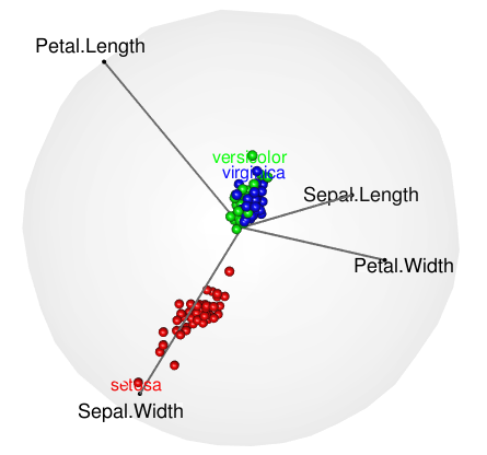
For small datasets with continuous values, function radialvis3d can be applied directly with options domrp = F and doGtrans = F. The 3D plot below are displayed for the (Fisher’s or Anderson’s) iris data. The dataset contains 50 flowers measurements for 4 variables, sepal length, sepal width, petal length and petal width which are represented by the 4 anchor points in the plot. Flowers come from each of 3 species, Iris setosa, Iris versicolor, and Iris virginica. Speicies groups are shown in different colors and tagged with name labels.

library(radviz3d)
data("iris")
radialvis3d(data = iris[, -5], cl = factor(iris$Species), domrp = F, doGtrans = F, 
            lwd = 2, alpha = 0.05, pradius = 0.025, class.labels = levels(iris$Species))

Display reduced datasets

For large datasets with continuous values, we use function radialvis3d with options doGtrans = F and domrp = T along with the number of principal components k specified by npc = k. The plot for a wine dataset are shown below. The dataset (reference link: ) contains 178 samples of three types of wines grown in a specific area of Italy. 13 chemical analyses were recorded for each sample.

radialvis3d(data = wine[, -14], cl = factor(wine[,14]), domrp = T, npc = 4, doGtrans = F, 
            lwd = 2, alpha = 0.05, pradius = 0.025, class.labels = levels(wine[,14]))
#> cumulative variance explained: 0.9913192 1 1 1 1 1 1 1 1 1 1 1 1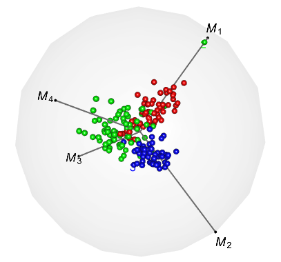

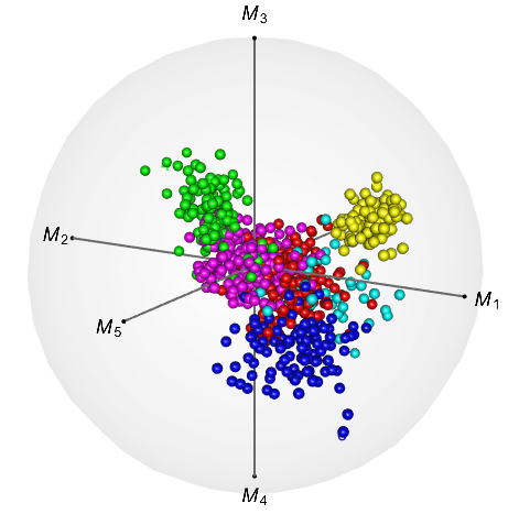
Display transformed datasets

Datasets with discrete values can be transformed using options doGtrans = T. (Currently, GDT is not applicable to categorical variables). Here we present an example for an Indic scripts dataset (reference link: ) which is on 116 different features from handwritten scripts of 11 Indic languages. A subset of 5 languages is chosen from 4 regions, namely Bangla (from the east), Gurmukhi (north), Gujarati (west), and Kannada and Malayalam (languages from the neighboring southern states of Karnataka and Kerala) and a sixth language (Urdu, with a distinct Persian script). Some of the features contains discrete values so the dataset is essentially of mixed attributes. We apply radialvis3d with GDT and MRP (npc = 6) to display for distinctiveness of samples from each languages.

radialvis3d(data = script[,-117], cl = class, domrp = T, npc = 6, doGtrans = T, 
            lwd = 2, alpha = 0.05, pradius = 0.025, class.labels = levels(class))
#> cumulative variance explained: 0.3707163 0.6445103 0.8170576 0.9416525 1 1 1 1 1 1 1 1 1 1 1 1 1 1 1 1 1 1 1 1 1 1 1 1 1 1 1 1 1 1 1 1 1 1 1 1 1 1 1 1 1 1