Type:	Package
Title:	Solving Mixed Model Equations in R
Version:	4.4.2
Date:	2025-05-25
Maintainer:	Giovanny Covarrubias-Pazaran <cova_ruber@live.com.mx>
Description:	Structural multivariate-univariate linear mixed model solver for estimation of multiple random effects with unknown variance-covariance structures (e.g., heterogeneous and unstructured) and known covariance among levels of random effects (e.g., pedigree and genomic relationship matrices) (Covarrubias-Pazaran, 2016 <doi:10.1371/journal.pone.0156744>; Maier et al., 2015 <doi:10.1016/j.ajhg.2014.12.006>; Jensen et al., 1997). REML estimates can be obtained using the Direct-Inversion Newton-Raphson and Direct-Inversion Average Information algorithms for the problems r x r (r being the number of records) or using the Henderson-based average information algorithm for the problem c x c (c being the number of coefficients to estimate). Spatial models can also be fitted using the two-dimensional spline functionality available.
Depends:	R (≥ 3.5.0), Matrix (≥ 1.1.1), methods, stats, MASS, crayon
LazyLoad:	yes
LazyData:	yes
License:	GPL-2 | GPL-3 [expanded from: GPL (≥ 2)]
Imports:	Rcpp (≥ 0.12.19)
BugReports:	https://github.com/covaruber/sommer/issues
URL:	https://github.com/covaruber/sommer
LinkingTo:	Rcpp, RcppArmadillo, RcppProgress
Suggests:	rmarkdown, knitr, plyr, parallel, orthopolynom, RSpectra, lattice, testthat (≥ 3.0.0)
VignetteBuilder:	knitr
Config/testthat/edition:	3
NeedsCompilation:	yes
Packaged:	2025-05-26 19:49:58 UTC; giovannycovarrubias
Author:	Giovanny Covarrubias-Pazaran [aut, cre]
Repository:	CRAN
Date/Publication:	2025-05-26 20:30:02 UTC

Additive relationship matrix

Description

Calculates the realized additive relationship matrix. Currently is the C++ implementation of van Raden (2008).

Usage

A.mat(X,min.MAF=0,return.imputed=FALSE)

Arguments

Details

For vanraden method: the marker matrix is centered by subtracting column means M= X - ms where ms is the coumn means. Then A=M M'/c, where c = \sum_k{d_k}/k, the mean value of the diagonal values of the M M' portion.

Value

If return.imputed = FALSE, the n \times n additive relationship matrix is returned.

If return.imputed = TRUE, the function returns a list containing

$A

the A matrix

$X

the imputed marker matrix

References

Endelman, J.B., and J.-L. Jannink. 2012. Shrinkage estimation of the realized relationship matrix. G3:Genes, Genomes, Genetics. 2:1405-1413. doi: 10.1534/g3.112.004259

Covarrubias-Pazaran G (2016) Genome assisted prediction of quantitative traits using the R package sommer. PLoS ONE 11(6): doi:10.1371/journal.pone.0156744

Examples

####=========================================####
#### random population of 200 lines with 1000 markers
####=========================================####
X <- matrix(rep(0,200*1000),200,1000)
for (i in 1:200) {
  X[i,] <- ifelse(runif(1000)<0.5,-1,1)
}

A <- A.mat(X)

####=========================================####
#### take a look at the Genomic relationship matrix 
#### (just a small part)
####=========================================####
# colfunc <- colorRampPalette(c("steelblue4","springgreen","yellow"))
# hv <- heatmap(A[1:15,1:15], col = colfunc(100),Colv = "Rowv")
# str(hv)

Autocorrelation matrix of order 1.

Description

Creates an autocorrelation matrix of order one with parameters specified.

Usage

AR1(x,rho=0.25)

Arguments

Details

Specially useful for constructing covariance structures for rows and ranges to capture better the spatial variation trends in the field. The rho value is assumed fixed and values of the variance component will be optimized through REML.

Value

If everything is defined correctly the function returns:

$nn

the correlation matrix

References

Covarrubias-Pazaran G (2016) Genome assisted prediction of quantitative traits using the R package sommer. PLoS ONE 11(6): doi:10.1371/journal.pone.0156744

Examples

x <- 1:4
R1 <- AR1(x,rho=.25)
image(R1)

data(DT_sleepstudy)
DT <- DT_sleepstudy
head(DT)

# define the correlation between Days
D = with(DT, AR1(Days, rho=0.5))
subs = unique(DT$Subject)
# define the correlation between Subjects
S = diag(length(subs))
rownames(S) <- colnames(S) <- subs
# make the kronecker product
DS = kronecker(D,S, make.dimnames = TRUE)
# form the covariance matrix between units 
# this is assumes correlation between timepoints
DT$ds <- paste(DT$Days, DT$Subject, sep=":")
DS <- DS[DT$ds, DT$ds]
colnames(DS) <- rownames(DS) <- paste0("u",1:nrow(DS))
# fit the residual model
head(DT)

fm2 <- mmes(Reaction ~ Days,
            random= ~ Subject, 
            rcov = ~vsm(ism(units), Gu=DS), # equivalent to Subject:ar1(Days)
            data=DT, tolParInv = 1e-6, verbose = FALSE)
summary(fm2)$varcomp

# the matrix D can take any form: AR1, ARMA, or a custom correlation matrix

Autocorrelation Moving average.

Description

Creates an ARMA matrix of order one with parameters specified.

Usage

ARMA(x, rho=0.25, lambda=0.25)

Arguments

Details

Specially useful for constructing covariance structures for rows and ranges to capture better the spatial variation trends in the field. The rho value is assumed fixed and values of the variance component will be optimized through REML.

Value

If everything is defined correctly the function returns:

$nn

the correlation matrix

References

Covarrubias-Pazaran G (2016) Genome assisted prediction of quantitative traits using the R package sommer. PLoS ONE 11(6): doi:10.1371/journal.pone.0156744

Examples

x <- 1:4
R1 <- ARMA(x,rho=.25,lambda=0.2)
image(R1)

Compound symmetry matrix

Description

Creates a compound symmetry matrix with parameters specified.

Usage

CS(x, rho=0.25)

Arguments

Details

Specially useful for constructing covariance structures for rows and ranges to capture better the spatial variation trends in the field. The rho value is assumed fixed and values of the variance component will be optimized through REML.

Value

If everything is defined correctly the function returns:

$nn

the correlation matrix

References

Covarrubias-Pazaran G (2016) Genome assisted prediction of quantitative traits using the R package sommer. PLoS ONE 11(6): doi:10.1371/journal.pone.0156744

Examples

x <- 1:4
R1 <- CS(x,rho=.25)
image(R1)

Dominance relationship matrix

Description

C++ implementation of the dominance matrix. Calculates the realized dominance relationship matrix. Can help to increase the prediction accuracy when 2 conditions are met; 1) The trait has intermediate to high heritability, 2) The population contains a big number of individuals that are half or full sibs (HS & FS).

Usage

D.mat(X,nishio=TRUE,min.MAF=0,return.imputed=FALSE)

Arguments

Details

The additive marker coefficients will be used to compute dominance coefficients as: Xd = 1-abs(X) for diploids.

For nishio method: the marker matrix is centered by subtracting column means M= Xd - ms where ms is the column means. Then A=M M'/c, where c = 2 \sum_k {p_k (1-p_k)}.

For su method: the marker matrix is normalized by subtracting row means M= Xd - 2pq where 2pq is the product of allele frequencies times 2. Then A=M M'/c, where c = 2 \sum_k {2pq_k (1-2pq_k)}.

Value

If return.imputed = FALSE, the n \times n additive relationship matrix is returned.

If return.imputed = TRUE, the function returns a list containing

$D

the D matrix

$imputed

the imputed marker matrix

References

Covarrubias-Pazaran G (2016) Genome assisted prediction of quantitative traits using the R package sommer. PLoS ONE 11(6): doi:10.1371/journal.pone.0156744

Nishio M and Satoh M. 2014. Including Dominance Effects in the Genomic BLUP Method for Genomic Evaluation. Plos One 9(1), doi:10.1371/journal.pone.0085792

Su G, Christensen OF, Ostersen T, Henryon M, Lund MS. 2012. Estimating Additive and Non-Additive Genetic Variances and Predicting Genetic Merits Using Genome-Wide Dense Single Nucleotide Polymorphism Markers. PLoS ONE 7(9): e45293. doi:10.1371/journal.pone.0045293

Examples

####=========================================####
#### EXAMPLE 1
####=========================================####
####random population of 200 lines with 1000 markers
X <- matrix(rep(0,200*1000),200,1000)
for (i in 1:200) {
  X[i,] <- sample(c(-1,0,0,1), size=1000, replace=TRUE)
}

D <- D.mat(X)

DT_augment design example.

Description

This dataset contains phenotpic data for one trait evaluated in the experimental design known as augmented design. This model allows to obtain BLUPs for genotypes that are unreplicated by dividing the field in blocks and replicating 'check genotypes' in the blocks and unreplicated genotypes randomly within the blocks. The presence of check genotypes (usually cultivars) allows the adjustment of unreplicated genotypes.

The column 'Plot' indicates the number of plot in the field The column 'Entry' is a numeric value for each entry The colum 'Genotype' is the name of the individual The column 'Block' is the replicate or big block The column TSW is the response variable The column check is an indicator column for checks (0) and non-checks (1) The column Check.Gen is an indicator column for checks (89,90,91) and non-checks (999)

The dataset has 3 unique checks (Ross=89, MF183=90, Starlight=91) and 50 entries.

Usage

data("DT_augment")

Format

The format is: chr "DT_augment"

Source

This data was generated by a potato study.

References

Covarrubias-Pazaran G (2016) Genome assisted prediction of quantitative traits using the R package sommer. PLoS ONE 11(6): doi:10.1371/journal.pone.0156744

See Also

The core functions of the package mmes

Examples

# ###=========================================####
# ### AUGMENTED DESIGN EXAMPLE
# ###=========================================####
# data(DT_augment)
# DT <- DT_augment
# head(DT)
# ####=========================================####
# #### fit the mixed model and check summary
# ####=========================================####
# mix1 <- mmes(TSW ~ Check.Gen,
#              random = ~ Block + Genotype:Check,
#              data=DT)
# summary(mix1)$varcomp

Blue Tit Data for a Quantitative Genetic Experiment

Description

a data frame with 828 rows and 7 columns, with variables tarsus length (tarsus) and colour (back) measured on 828 individuals (animal). The mother of each is also recorded (dam) together with the foster nest (fosternest) in which the chicks were reared. The date on which the first egg in each nest hatched (hatchdate) is recorded together with the sex (sex) of the individuals.

Usage

data("DT_btdata")

Format

The format is: chr "DT_btdata"

References

Covarrubias-Pazaran G (2016) Genome assisted prediction of quantitative traits using the R package sommer. PLoS ONE 11(6): doi:10.1371/journal.pone.0156744

See Also

The core functions of the package mmes

Examples

# ####=========================================####
# #### For CRAN time limitations most lines in the 
# #### examples are silenced with one '#' mark, 
# #### remove them and run the examples
# ####=========================================####
# ####=========================================####
# ####=========================================####
# #### EXAMPLE 1
# #### simple example
# ####=========================================####
# ####=========================================####
# data(DT_btdata)
# DT <- DT_btdata
# head(DT)
# mix4 <- mmes(tarsus ~ sex,
#              random = ~ dam + fosternest,
#              rcov=~units,
#              data = DT)
# summary(mix4)$varcomp

# MULTI-TRAIT EXAMPLE
# head(DT)
# DT2 <- stackTrait(DT, traits = c("tarsus","back"))
# head(DT2$long)
# DT2$long=DT2$long[with(DT2$long, order(trait)), ]
# 
# mix3 <- mmes(valueS ~ trait:sex - 1, henderson=TRUE,
#                 random = ~ vsm(usm(trait),ism(dam)) +  
#                            vsm(usm(trait), ism(fosternest)),
#                 rcov= ~ vsm(dsm(trait),ism(units)),
#                 data = DT2$long)
# 
# 
# summary(mix3)$varcomp
# #### calculate the genetic correlation
# cov2cor(mix3$theta[[1]])
# cov2cor(mix3$theta[[2]])

Corn crosses and markers

Description

This dataset contains phenotpic data for plant height and grain yield for 100 out of 400 possible hybrids originated from 40 inbred lines belonging to 2 heterotic groups, 20 lines in each, 1600 rows exist for the 400 possible hybrids evaluated in 4 locations but only 100 crosses have phenotypic information. The purpose of this data is to show how to predict the other 300 crosses.

The data contains 3 elements. The first is the phenotypic data and the parent information for each cross evaluated in the 4 locations. 1200 rows should have missing data but the 100 crosses performed were chosen to be able to estimate the GCA and SCA effects of everything.

The second element of the data set is the phenotypic data and other relevant information for the 40.

The third element is the genomic relationship matrix for the 40 inbred lines originated from 511 SNP markers and calculated using the A.mat function.

Usage

data("DT_cornhybrids")

Format

The format is: chr "DT_cornhybrids"

Source

This data was generated by a corn study.

References

Covarrubias-Pazaran G (2016) Genome assisted prediction of quantitative traits using the R package sommer. PLoS ONE 11(6): doi:10.1371/journal.pone.0156744

See Also

The core functions of the package mmes

Examples

# ####=========================================####
# #### For CRAN time limitations most lines in the 
# #### examples are silenced with one '#' mark, 
# #### remove them and run the examples using
# #### command + shift + C |OR| control + shift + C
# ####=========================================####
# 
# data(DT_cornhybrids)
# DT <- DT_cornhybrids
# DTi <- DTi_cornhybrids
# GT <- GT_cornhybrids
# hybrid2 <- DT # extract cross data
# A <- GT
# K1 <- A[levels(hybrid2$GCA1), levels(hybrid2$GCA1)]; dim(K1)
# K2 <- A[levels(hybrid2$GCA2), levels(hybrid2$GCA2)]; dim(K2)
# S <- kronecker(K1, K2) ; dim(S)
# rownames(S) <- colnames(S) <- levels(hybrid2$SCA)
# 
# ans <- mmes(Yield ~ Location,
#              random = ~ vsm(ism(GCA1),Gu=K1) + vsm(ism(GCA2),Gu=K2), # + vsm(ism(SCA),Gu=S),
#              rcov=~units,
#              data=hybrid2)
# summary(ans)$varcomp
# 
# ## mmec uses the inverse of the relationship matrix
# K1i <- solve(K1 + diag(1e-4,ncol(K1),ncol(K1)))
# K1i <- as(as(as( K1i,  "dMatrix"), "generalMatrix"), "CsparseMatrix")
# attr(K1i, 'inverse')=TRUE 
# K2i <- solve(K2 + diag(1e-4,ncol(K2),ncol(K2)))
# K2i <- as(as(as( K2i,  "dMatrix"), "generalMatrix"), "CsparseMatrix")
# attr(K2i, 'inverse')=TRUE 
# Si <- solve(S + diag(1e-4,ncol(S),ncol(S)))
# Si <- as(as(as( Si,  "dMatrix"), "generalMatrix"), "CsparseMatrix")
# attr(Si, 'inverse')=TRUE 
# ans2 <- mmes(Yield ~ Location,
#              random = ~ vsm(ism(GCA1),Gu=K1i) + vsm(ism(GCA2),Gu=K2i), # + vsm(ism(SCA),Gu=Si),
#              henderson=TRUE,
#              rcov=~units,
#              data=hybrid2)
# summary(ans2)$varcomp

Genotypic and Phenotypic data for a CP population

Description

A CP population or F1 cross is the designation for a cross between 2 highly heterozygote individuals; i.e. humans, fruit crops, bredding populations in recurrent selection.

This dataset contains phenotpic data for 363 siblings for an F1 cross. These are averages over 2 environments evaluated for 4 traits; color, yield, fruit average weight, and firmness. The columns in the CPgeno file are the markers whereas the rows are the individuals. The CPpheno data frame contains the measurements for the 363 siblings, and as mentioned before are averages over 2 environments.

Usage

data("DT_cpdata")

Format

The format is: chr "DT_cpdata"

Source

This data was simulated for fruit breeding applications.

References

Covarrubias-Pazaran G (2016) Genome assisted prediction of quantitative traits using the R package sommer. PLoS ONE 11(6): doi:10.1371/journal.pone.0156744

See Also

The core functions of the package mmes

Examples

# ####=========================================####
# #### For CRAN time limitations most lines in the
# #### examples are silenced with one '#' mark,
# #### remove them and run the examples using
# #### command + shift + C |OR| control + shift + C
# ####=========================================####
#
# data(DT_cpdata)
# DT <- DT_cpdata
# GT <- GT_cpdata
# MP <- MP_cpdata
# #### create the variance-covariance matrix
# A <- A.mat(GT) # additive relationship matrix
# #### look at the data and fit the model
# head(DT)
# mix1 <- mmes(Yield~1, henderson=FALSE,
#               random=~vsm(ism(id),Gu=A)
#                       + Rowf + Colf,
#               rcov=~units,
#               data=DT)
# summary(mix1)$varcomp
#
# ## mmec uses the inverse of the relationship matrix
# Ai <- solve(A + diag(1e-4,ncol(A),ncol(A)))
# Ai <- as(as(as( Ai,  "dMatrix"), "generalMatrix"), "CsparseMatrix")
# attr(Ai, 'inverse')=TRUE 
# mix2 <- mmes(Yield~1, henderson=TRUE,
#               random=~vsm(ism(id),Gu=Ai)
#                       + Rowf + Colf,
#               rcov=~units,
#               data=DT)
# summary(mix2)$varcomp
#
# vg <- summary(mix2)$varcomp[1,1] # genetic variance
# G <- A*vg # genetic variance-covariance
# Ci <- mix2$Ci # coefficient matrix
# ind <- as.vector(mix2$partitions$`vsm(ism(id), Gu = Ai)`)
# ind <- seq(ind[1],ind[2])
# Ctt <- Ci[ind,ind] # portion of Ci for genotypes
# R2 <- (G - Ctt)/G # reliability matrix
# mean(diag(R2)) # average reliability of the trial
# ####====================####
# #### multivariate model ####
# ####     2 traits       ####
# ####====================####
# head(DT)
# DT2 <- stackTrait(DT, traits = c("color","Yield"))
# head(DT2$long)
# A <- A.mat(GT) # additive relationship matrix
# # if using mmes=TRUE you need to provide the inverse
# Ai <- solve(A + diag(1e-4,ncol(A),ncol(A)))
# Ai <- as(as(as( Ai,  "dMatrix"), "generalMatrix"), "CsparseMatrix")
# attr(Ai, 'inverse')=TRUE 
# #### be patient take some time
# ansm <- mmes( valueS ~ trait, # henderson=TRUE,
#                random=~ vsm(usm(trait), ism(id), Gu=A),
#                rcov=~ vsm(dsm(trait), ism(units)),
#                data=DT2$long)
# cov2cor(ansm$theta[[1]])

Broad sense heritability calculation.

Description

This dataset contains phenotpic data for 41 potato lines evaluated in 3 environments in an RCBD design. The phenotypic trait is tuber quality and we show how to obtain an estimate of DT_example for the trait.

Usage

data("DT_example")

Format

The format is: chr "DT_example"

Source

This data was generated by a potato study.

References

Covarrubias-Pazaran G (2016) Genome assisted prediction of quantitative traits using the R package sommer. PLoS ONE 11(6): doi:10.1371/journal.pone.0156744

See Also

The core functions of the package mmes

Examples

####=========================================####
#### For CRAN time limitations most lines in the 
#### examples are silenced with one '#' mark, 
#### remove them and run the examples
####=========================================####
####=========================================####
#### EXAMPLES
#### Different models with sommer
####=========================================####

data(DT_example)
DT <- DT_example
A <- A_example
head(DT)

####=========================================####
#### Univariate homogeneous variance models  ####
####=========================================####

## Compound simmetry (CS) model
ans1 <- mmes(Yield~Env,
             random= ~ Name + Env:Name,
             rcov= ~ units,
             data=DT)
summary(ans1)$varcomp

# ####===========================================####
# #### Univariate heterogeneous variance models  ####
# ####===========================================####
# 
# ## Compound simmetry (CS) + Diagonal (DIAG) model
# DT=DT[with(DT, order(Env)), ]
# ans2 <- mmes(Yield~Env,
#              random= ~Name + vsm(dsm(Env),ism(Name)),
#              rcov= ~ vsm(dsm(Env),ism(units)),
#              data=DT)
# summary(ans2)

Data for different experimental designs

Description

The following data is a list containing data frames for different type of experimental designs relevant in plant breeding:

1) Augmented designs (2 examples)

2) Incomplete block designs (1 example)

3) Split plot design (2 examples)

4) Latin square designs (1 example)

5) North Carolina designs I,II and III

How to fit each is shown at the Examples section. This may help you get introduced to experimental designs relevant to plant breeding. Good luck.

Format

Different based on the design.

Source

Datasets and more detail about them can be found in the agricolae package. Here we just show the datasets and how to analyze them using the sommer package.

References

Covarrubias-Pazaran G (2016) Genome assisted prediction of quantitative traits using the R package sommer. PLoS ONE 11(6): doi:10.1371/journal.pone.0156744

Examples

# #### =================================== ####
# #### ===== Augmented Block Design 1 ==== ####
# #### =================================== ####
# data(DT_expdesigns)
# DT <- DT_expdesigns
# names(DT)
# data1 <- DT$au1
# head(data1)
# ## response variable: "yield"
# ## check indicator: "entryc" ('nc' for all unreplicated, but personal.name for checks)
# ## blocking factor: "block"
# ## treatments, personal names for replicated and non-replicated: "trt"
# ## check no check indicator: "new"
# mix1 <- mmes(yield~entryc,
#              random=~block+trt,
#              rcov=~units, 
#              data=data1)
# summary(mix1)$varcomp

Full diallel data for corn hybrids

Description

This dataset contains phenotpic data for 36 winter bean hybrids, coming from a full diallel design and evaluated for 9 traits. The column male and female origin columns are included as well.

Usage

data("DT_fulldiallel")

Format

The format is: chr "DT_fulldiallel"

Source

This data was generated by a winter bean study and originally included in the agridat package.

References

Covarrubias-Pazaran G (2016) Genome assisted prediction of quantitative traits using the R package sommer. PLoS ONE 11(6): doi:10.1371/journal.pone.0156744

See Also

The core functions of the package mmes

Examples

####=========================================####
#### For CRAN time limitations most lines in the
#### examples are silenced with one '#' mark,
#### remove them and run the examples
####=========================================####
data(DT_fulldiallel)
DT <- DT_fulldiallel
head(DT)
mix <- mmes(stems~1, random=~female+male, data=DT)
summary(mix)

Gryphon data from the Journal of Animal Ecology

Description

This is a dataset that was included in the Journal of animal ecology by Wilson et al. (2010; see references) to help users understand how to use mixed models with animal datasets with pedigree data.

The dataset contains 3 elements:

gryphon; variables indicating the animal, the mother of the animal, sex of the animal, and two quantitative traits named 'BWT' and 'TARSUS'.

pedi; dataset with 2 columns indicating the sire and the dam of the animals contained in the gryphon dataset.

A; additive relationship matrix formed using the 'getA()' function used over the pedi dataframe.

Usage

data("DT_gryphon")

Format

The format is: chr "DT_gryphon"

Source

This data comes from the Journal of Animal Ecology. Please, if using this data cite Wilson et al. publication. If using our mixed model solver please cite Covarrubias' publication.

References

Wilson AJ, et al. (2010) An ecologist's guide to the animal model. Journal of Animal Ecology 79(1): 13-26.

Covarrubias-Pazaran G (2016) Genome assisted prediction of quantitative traits using the R package sommer. PLoS ONE 11(6): doi:10.1371/journal.pone.0156744

See Also

The core functions of the package mmes

Examples

####=========================================####
#### For CRAN time limitations most lines in the 
#### examples are silenced with one '#' mark, 
#### remove them and run the examples using
#### command + shift + C |OR| control + shift + C
####=========================================####
# data(DT_gryphon)
# DT <- DT_gryphon
# A <- A_gryphon
# P <- P_gryphon
# #### look at the data
# head(DT)
# #### fit the model with no fixed effects (intercept only)
# mix1 <- mmes(BWT~1,
#              random=~vsm(ism(ANIMAL),Gu=A),
#              rcov=~units,
#              data=DT)
# summary(mix1)$varcomp
# 
# ## mmes algorithm uses the inverse of the relationship matrix
# Ai <- solve(A + diag(1e-4,ncol(A),ncol(A)))
# Ai <- as(as(as( Ai,  "dMatrix"), "generalMatrix"), "CsparseMatrix")
# attr(Ai, 'inverse')=TRUE 
# ####====================####
# #### multivariate model ####
# ####     2 traits       ####
# ####====================####
# head(DT)
# DT2 <- stackTrait(DT, traits = c("BWT","TARSUS"))
# head(DT2$long)
# 
# # #### fit the multivariate model with no fixed effects (intercept only)
# mix2 <- mmes(valueS~trait, henderson=FALSE, 
#              random=~vsm(usm(trait),ism(ANIMAL),Gu=A),
#              rcov=~vsm(dsm(trait),ism(units)),
#              data=DT2$long)
# summary(mix2)$varcomp
# cov2cor(mix2$theta[[1]])

Broad sense heritability calculation.

Description

This dataset contains phenotpic data for 41 potato lines evaluated in 5 locations across 3 years in an RCBD design. The phenotypic trait is tuber quality and we show how to obtain an estimate of DT_h2 for the trait.

Usage

data("DT_h2")

Format

The format is: chr "DT_h2"

Source

This data was generated by a potato study.

References

Covarrubias-Pazaran G (2016) Genome assisted prediction of quantitative traits using the R package sommer. PLoS ONE 11(6): doi:10.1371/journal.pone.0156744

See Also

The core functions of the package mmes

Examples

####=========================================####
#### For CRAN time limitations most lines in the 
#### examples are silenced with one '#' mark, 
#### remove them and run the examples
####=========================================####
data(DT_h2)
DT <- DT_h2
head(DT)
####=========================================####
#### fit the mixed model (very heavy model)
####=========================================####
# DT=DT[with(DT, order(Env)), ]
# ans1 <- mmes(y~Env, henderson=TRUE,
#               random=~vsm(dsm(Env),ism(Name)) + vsm(dsm(Env),ism(Block)),
#               rcov=~vsm(dsm(Env),ism(units)),
#               data=DT)
# summary(ans1)$varcomp
# 

half diallel data for corn hybrids

Description

This dataset contains phenotpic data for 21 corn hybrids, with 2 technical repetitions, coming from a half diallel design and evaluated for sugar content. The column geno indicates the hybrid and male and female origin columns are included as well.

Usage

data("DT_halfdiallel")

Format

The format is: chr "DT_halfdiallel"

Source

This data was generated by a corn study.

References

Covarrubias-Pazaran G (2016) Genome assisted prediction of quantitative traits using the R package sommer. PLoS ONE 11(6): doi:10.1371/journal.pone.0156744

See Also

The core functions of the package mmes

Examples

####=========================================####
#### For CRAN time limitations most lines in the 
#### examples are silenced with one '#' mark, 
#### remove them and run the examples
####=========================================####

data("DT_halfdiallel")
DT <- DT_halfdiallel
head(DT)
DT$femalef <- as.factor(DT$female)
DT$malef <- as.factor(DT$male)
DT$genof <- as.factor(DT$geno)

A <- diag(7); colnames(A) <- rownames(A) <- 1:7;A # if you want to provide a covariance matrix
#### model using overlay
modh <- mmes(sugar~1, 
             random=~vsm(ism(overlay(femalef,malef, sparse = FALSE)), Gu=A) 
             + genof,
             data=DT)
summary(modh)$varcomp

# if ussing mmes=TRUE provide Gu with inverses and give more iterations
# Ai <- solve(A + diag(1e-4,ncol(A),ncol(A)))
# Ai <- as(as(as( Ai,  "dMatrix"), "generalMatrix"), "CsparseMatrix")
# attr(Ai, 'inverse')=TRUE 

Data to fit indirect genetic effects.

Description

This dataset contains phenotpic data for 98 individuals where they are measured with the purpose of identifying the effect of the neighbour in a focal individual.

Usage

data("DT_ige")

Format

The format is: chr "DT_ige"

Source

This data was masked from a shared study.

References

Covarrubias-Pazaran G (2016) Genome assisted prediction of quantitative traits using the R package sommer. PLoS ONE 11(6): doi:10.1371/journal.pone.0156744

See Also

The core functions of the package mmes

Examples

####=========================================####
#### For CRAN time limitations most lines in the 
#### examples are silenced with one '#' mark, 
#### remove them and run the examples
####=========================================####
####=========================================####
#### EXAMPLES
#### Different models with sommer
####=========================================####

data(DT_ige)
DT <- DT_ige
# # Indirect genetic effects model without covariance between DGE and IGE
# modIGE <- mmes(trait ~ block, dateWarning = FALSE,
#                random = ~ focal + neighbour,
#                rcov = ~ units, nIters=100,
#               data = DT)
# summary(modIGE)$varcomp
# pmonitor(modIGE)
# 
# # Indirect genetic effects model with covariance between DGE and IGE using relationship matrices
# modIGE <- mmes(trait ~ block, dateWarning = FALSE,
#                random = ~ covm( vsm(ism(focal)), vsm(ism(neighbour)) ),
#                rcov = ~ units, nIters=100,
#               data = DT)
# summary(modIGE)$varcomp
# pmonitor(modIGE)
# 
# # form relationship matrix
# Ai <- solve(A_ige + diag(1e-5, nrow(A_ige),nrow(A_ige) ))
# Ai <- as(as(as( Ai,  "dMatrix"), "generalMatrix"), "CsparseMatrix")
# attr(Ai, 'inverse')=TRUE 
# # Indirect genetic effects model with covariance between DGE and IGE using relationship matrices
# modIGE <- mmes(trait ~ block, dateWarning = FALSE,
#                random = ~ covm( vsm(ism(focal), Gu=Ai), vsm(ism(neighbour), Gu=Ai) ),
#                rcov = ~ units, nIters=100,
#               data = DT)
# summary(modIGE)$varcomp
# pmonitor(modIGE)

Simulated data for random regression

Description

A data frame with 4 columns; SUBJECT, X, Xf and Y to show how to use the Legendre polynomials in the mmes function using a numeric variable X and a response variable Y.

Usage

data("DT_legendre")

Format

The format is: chr "DT_legendre"

Source

This data was simulated for fruit breeding applications.

References

Covarrubias-Pazaran G (2016) Genome assisted prediction of quantitative traits using the R package sommer. PLoS ONE 11(6): doi:10.1371/journal.pone.0156744

See Also

The core functions of the package mmes

Examples

####=========================================####
#### For CRAN time limitations most lines in the 
#### examples are silenced with one '#' mark, 
#### remove them and run the examples using
#### command + shift + C |OR| control + shift + C
####=========================================####
# you need to install the orthopolynom library to do random regression models
# library(orthopolynom)
# data(DT_legendre)
# DT <- DT_legendre
# mRR2<-mmes(Y~ 1 + Xf
#            , random=~ vsm(usm(leg(X,1)),ism(SUBJECT))
#            , rcov=~units
#            , data=DT)
# summary(mRR2)$varcomp

Full diallel data for corn hybrids

Description

This dataset contains phenotpic data for 36 winter bean hybrids, coming from a full diallel design and evaluated for 9 traits. The column male and female origin columns are included as well.

Usage

data("DT_mohring")

Format

The format is: chr "DT_mohring"

Source

This data was generated by a winter bean study and originally included in the agridat package.

References

Covarrubias-Pazaran G (2016) Genome assisted prediction of quantitative traits using the R package sommer. PLoS ONE 11(6): doi:10.1371/journal.pone.0156744

See Also

The core functions of the package mmes

Examples

# ####=========================================####
# #### For CRAN time limitations most lines in the
# #### examples are silenced with one '#' mark,
# #### remove them and run the examples
# ####=========================================####
# data(DT_mohring)
# DT <- DT_mohring
# head(DT)
# DT2 <- add.diallel.vars(DT,par1="Par1", par2="Par2")
# head(DT2)
# # is.cross denotes a hybrid (1)
# # is.self denotes an inbred (1)
# # cross.type denotes one way (-1, e.g. AxB) and reciprocal (1, e.g., BxA) and no cross (0)
# # cross.id denotes the name of the cross (same name for direct & reciprocal)
#
# # GRIFFING MODEL 2 with reciprocal effects ###########################
#
# mod1hb <- mmes(Ftime ~ 1, data=DT2,
#                random = ~ Block
#                # GCA male & female overlayed
#                + vsm(ism(overlay(Par1, Par2)))
#                # SCA effects (includes cross and selfs)
#                + cross.id
#                # SCAR reciprocal effects (remaining variance in crosses; 
#                # if zero there's no reciprocal effects)
#                + vsm(dsm(cross.type), ism(cross.id)) )
# summary(mod1hb)$varcomp
#
# ##                                    VarComp VarCompSE   Zratio
# ## Block.Ftime-Ftime                  0.00000   9.32181 0.000000
# ## overlay(Par1, Par2).Ftime-Ftime 1276.73089 750.17269 1.701916
# ## cross.id.Ftime-Ftime            1110.99090 330.16921 3.364914
# ## cross.id:cross.type.Ftime-Ftime   66.02295  49.26876 1.340057
# ## units.Ftime-Ftime                418.47949  74.56442 5.612321
# ##
# # GRIFFING MODEL 2, no reciprocal effects ##############################
#
# mod1h <- mmes(Ftime ~ Block + is.cross, data=DT2, nIters = 50,
#               random = ~
#                 # GCA effects for all (hybrids and inbreds)
#                 vsm(ism(overlay(Par1, Par2)))
#               # GCA effect (calculated only in hybrids; remaining variance)
#               + vsm(ism(is.cross),ism(overlay(Par1, Par2)))
#               # SCA effect (calculated in hybrids only)
#               + vsm(ism(is.cross), ism(cross.id))
#               )
# summary(mod1h)$varcomp
#
# ##                                           VarComp  VarCompSE   Zratio
# ## overlay(Par1, Par2).Ftime-Ftime          2304.1781 1261.63193 1.826347
# ## overlay(Par1, Par2):is.cross.Ftime-Ftime  613.6040  402.74347 1.523560
# ## cross.id:is.cross.Ftime-Ftime             340.7030  148.56225 2.293335
# ## units.Ftime-Ftime                         501.6275   74.36075 6.745864
# ##
# # GRIFFING MODEL 3, no reciprocal effects ###############################
#
# mod1h <- mmes(Ftime ~ Block + is.cross, data=DT2, nIters = 100,
#               random = ~
#                 # GCAC (only for hybrids)
#                 vsm(ism(is.cross),ism(overlay(Par1, Par2)))
#               # male GCA (only for inbreds)
#               + vsm(ism(is.self),ism(Par1))
#               # SCA (for hybrids only)
#               + vsm(ism(is.cross), ism(cross.id))
#               )
# summary(mod1h)$varcomp
# ##                                           VarComp  VarCompSE   Zratio
# ## overlay(Par1, Par2):is.cross.Ftime-Ftime  927.7895  537.91218 1.724797
# ## Par1:is.self.Ftime-Ftime                 9960.9247 5456.58188 1.825488
# ## cross.id:is.cross.Ftime-Ftime             341.4567  148.53667 2.298804
# ## units.Ftime-Ftime                         498.5974   73.92066 6.745035
# ##
# # GRIFFING MODEL 2, with reciprocal effects #############################
# # In Mohring: mixed model 3 reduced
#
# mod1h <- mmes(Ftime ~ Block + is.cross, data=DT2, nIters = 100,
#               random = ~
#                 # GCAC (for hybrids only)
#                 vsm(ism(is.cross),ism(overlay(Par1, Par2)))
#               # male GCA (for selfs only)
#               + vsm(ism(is.self),ism(Par1))
#               # SCA (for hybrids only)
#               + vsm(ism(is.cross), ism(cross.id))
#               # SCAR reciprocal effects (remaning SCA variance)
#               + vsm(ism(cross.type), ism(cross.id))
#               )
# summary(mod1h)$varcomp
#
# ##                                             VarComp  VarCompSE   Zratio
# ## overlay(Par1, Par2):is.cross.Ftime-Ftime   927.78742  537.89981 1.724833
# ## Par1:is.self.Ftime-Ftime                 10001.78854 5456.47578 1.833013
# ## cross.id:is.cross.Ftime-Ftime              361.89712  148.54264 2.436318
# ## cross.id:cross.type.Ftime-Ftime             66.43695   49.24492 1.349113
# ## units.Ftime-Ftime                          416.82960   74.27202 5.612203
# ##
# # GRIFFING MODEL 3, with RGCA + RSCA ####################################
# # In Mohring: mixed model 3
#
# mod1h <- mmes(Ftime ~ Block + is.cross, data=DT2,nIters = 100,
#               random = ~
#                 # GCAC (for hybrids only)
#                 vsm(ism(is.cross),ism(overlay(Par1, Par2)))
#               # RGCA: exclude selfs (to identify reciprocal GCA effects)
#               + vsm(ism(cross.type),ism(overlay(Par1, Par2)))
#               # male GCA (for selfs only)
#               + vsm(ism(is.self),ism(Par1))
#               # SCA (for hybrids only)
#               + vsm(ism(is.cross), ism(cross.id))
#               # SCAR: exclude selfs (if zero there's no reciprocal SCA effects)
#               + vsm(ism(cross.type), ism(cross.id))
#               )
# summary(mod1h)$varcomp
#
# ##                                            VarComp  VarCompSE    Zratio
# ## overlay(Par1, Par2):is.cross.Ftime-Ftime   927.7843  537.88164 1.7248857
# ## Par1:is.self.Ftime-Ftime                 10001.7570 5456.30125 1.8330654
# ## cross.id:is.cross.Ftime-Ftime              361.8958  148.53670 2.4364068
# ## overlay(Par1, Par2):cross.type.Ftime-Ftime  17.9799   19.92428 0.9024114
# ## cross.id:cross.type.Ftime-Ftime             30.9519   46.43908 0.6665054
# ## units.Ftime-Ftime                         416.09922  447.2101 0.93043333

Genotypic and Phenotypic data for a potato polyploid population

Description

This dataset contains phenotpic data for 18 traits measured in 187 individuals from a potato diversity panel. In addition contains genotypic data for 221 individuals genotyped with 3522 SNP markers. Please if using this data for your own research make sure you cite Rosyara's (2015) publication (see References).

Usage

data("DT_polyploid")

Format

The format is: chr "DT_polyploid"

Source

This data was extracted from Rosyara (2016).

References

If using this data for your own research please cite:

Rosyara Umesh R., Walter S. De Jong, David S. Douches, Jeffrey B. Endelman. Software for genome-wide association studies in autopolyploids and its application to potato. The Plant Genome 2015.

Covarrubias-Pazaran G (2016) Genome assisted prediction of quantitative traits using the R package sommer. PLoS ONE 11(6): doi:10.1371/journal.pone.0156744

See Also

The core functions of the package mmes

Examples

####=========================================####
#### For CRAN time limitations most lines in the 
#### examples are silenced with one '#' mark, 
#### remove them and run the examples using
#### command + shift + C |OR| control + shift + C
####=========================================####

data(DT_polyploid)
# DT <- DT_polyploid
# GT <- GT_polyploid
# MP <- MP_polyploid
# ####=========================================####
# ####### convert markers to numeric format
# ####=========================================####
# numo <- atcg1234(data=GT, ploidy=4);
# numo$M[1:5,1:5];
# numo$ref.allele[,1:5]
# 
# ###=========================================####
# ###### plants with both genotypes and phenotypes
# ###=========================================####
# common <- intersect(DT$Name,rownames(numo$M))
# 
# ###=========================================####
# ### get the markers and phenotypes for such inds
# ###=========================================####
# marks <- numo$M[common,]; marks[1:5,1:5]
# DT2 <- DT[match(common,DT$Name),];
# DT2 <- as.data.frame(DT2)
# DT2[1:5,]
# 
# ###=========================================####
# ###### Additive relationship matrix, specify ploidy
# ###=========================================####
# A <- A.mat(marks)
# D <- D.mat(marks)
# ###=========================================####
# ### run as mixed model
# ###=========================================####
# ans <- mmes(tuber_shape~1,
#             random=~vsm(ism(Name), Gu=A),
#             data=DT2)
# summary(ans)$varcomp
# # if using mmes=TRUE provide Gu as inverse
# Ai <- solve(A + diag(1e-4,ncol(A),ncol(A)))
# Ai <- as(as(as( Ai,  "dMatrix"), "generalMatrix"), "CsparseMatrix")
# attr(Ai, 'inverse')=TRUE 

Rice lines dataset

Description

Information from a collection of 413 rice lines. The DT_rice data set is from Rice Diversity Org. Program. The lines are genotyped with 36,901 SNP markers and phenotyped for more than 30 traits. This data set was included in the package to play with it. If using it for your research make sure you cite the original publication from Zhao et al.(2011).

Usage

  data(DT_rice)

Format

RicePheno contains the phenotypes RiceGeno contains genotypes letter code RiceGenoN contains the genotypes in numerical code using atcg1234 converter function

Source

Rice Diversity Organization http://www.ricediversity.org/data/index.cfm.

References

Keyan Zhao, Chih-Wei Tung, Georgia C. Eizenga, Mark H. Wright, M. Liakat Ali, Adam H. Price, Gareth J. Norton, M. Rafiqul Islam, Andy Reynolds, Jason Mezey, Anna M. McClung, Carlos D. Bustamante & Susan R. McCouch (2011). Genome-wide association mapping reveals a rich genetic architecture of complex traits in Oryza sativa. Nat Comm 2:467 DOI: 10.1038/ncomms1467, Published Online 13 Sep 2011.

See Also

The core functions of the package mmes

Examples

####=========================================####
#### For CRAN time limitations most lines in the 
#### examples are silenced with one '#' mark, 
#### remove them and run the examples using
#### command + shift + C |OR| control + shift + C
####=========================================####
data(DT_rice)
# DT <- DT_rice
# GT <- GT_rice
# GTn <- GTn_rice
# head(DT)
# M <- atcg1234(GT)
# A <- A.mat(M$M)
# mix <- mmes(Protein.content~1,
#             random = ~vsm(ism(geno), Gu=A) + geno,
#             rcov=~units,
#             data=DT)
# summary(mix)$varcomp
# # if using henderson=TRUE provide Gu as inverse
# Ai <- solve(A + diag(1e-6,ncol(A),ncol(A)))
# Ai <- as(as(as( Ai,  "dMatrix"), "generalMatrix"), "CsparseMatrix")
# attr(Ai, 'inverse')=TRUE 

Reaction times in a sleep deprivation study

Description

The average reaction time per day for subjects in a sleep deprivation study. On day 0 the subjects had their normal amount of sleep. Starting that night they were restricted to 3 hours of sleep per night. The observations represent the average reaction time on a series of tests given each day to each subject. Data from sleepstudy to see how lme4 models can be translated in sommer.

Usage

data("DT_sleepstudy")

Format

The format is: chr "DT_sleepstudy"

Source

These data are from the study described in Belenky et al. (2003), for the sleep deprived group and for the first 10 days of the study, up to the recovery period.

References

Covarrubias-Pazaran G (2016) Genome assisted prediction of quantitative traits using the R package sommer. PLoS ONE 11(6): doi:10.1371/journal.pone.0156744

Gregory Belenky et al. (2003) Patterns of performance degradation and restoration during sleep restrictions and subsequent recovery: a sleep dose-response study. Journal of Sleep Research 12, 1-12.

See Also

The core functions of the package mmes

Examples

####=========================================####
#### For CRAN time limitations most lines in the
#### examples are silenced with one '#' mark,
#### remove them and run the examples
####=========================================####
# library(lme4)
data(DT_sleepstudy)
DT <- DT_sleepstudy
head(DT)
##################################
## lme4
# fm1 <- lmer(Reaction ~ Days + (1 | Subject), data=DT)
# vc <- VarCorr(fm1); print(vc,comp=c("Variance"))
## sommer
fm2 <- mmes(Reaction ~ Days,
            random= ~ Subject, 
            data=DT, tolParInv = 1e-6, verbose = FALSE)
summary(fm2)$varcomp

##################################
## lme4
# fm1 <- lmer(Reaction ~ Days + (Days || Subject), data=DT)
# vc <- VarCorr(fm1); print(vc,comp=c("Variance"))
## sommer
fm2 <- mmes(Reaction ~ Days,
            random= ~ Subject + vsm(ism(Days), ism(Subject)), 
            data=DT, tolParInv = 1e-6, verbose = FALSE)
summary(fm2)$varcomp

##################################
## lme4
# fm1 <- lmer(Reaction ~ Days + (Days | Subject), data=DT)
# vc <- VarCorr(fm1); print(vc,comp=c("Variance"))
## sommer
## no equivalence in sommer to find the correlation between the 2 vc
## this is the most similar which is equivalent to (intercept || slope)
fm2 <- mmes(Reaction ~ Days,
            random= ~ Subject + vsm(ism(Days), ism(Subject)), 
            data=DT, tolParInv = 1e-6, verbose = FALSE)
summary(fm2)$varcomp

##################################
## lme4
# fm1 <- lmer(Reaction ~ Days + (0 + Days | Subject), data=DT)
# vc <- VarCorr(fm1); print(vc,comp=c("Variance"))
## sommer
fm2 <- mmes(Reaction ~ Days,
            random= ~ vsm(ism(Days), ism(Subject)), 
            data=DT, tolParInv = 1e-6, verbose = FALSE)
summary(fm2)$varcomp

Genotypic and Phenotypic data from single cross hybrids (Technow et al.,2014)

Description

This dataset contains phenotpic data for 2 traits measured in 1254 single cross hybrids coming from the cross of Flint x Dent heterotic groups. In addition contains the genotipic data (35,478 markers) for each of the 123 Dent lines and 86 Flint lines. The purpose of this data is to demosntrate the prediction of unrealized crosses (9324 unrealized crosses, 1254 evaluated, total 10578 single crosses). We have added the additive relationship matrix (A) but can be easily obtained using the A.mat function on the marker data. Please if using this data for your own research cite Technow et al. (2014) publication (see References).

Usage

data("DT_technow")

Format

The format is: chr "DT_technow"

Source

This data was extracted from Technow et al. (2014).

References

If using this data for your own research please cite:

Technow et al. 2014. Genome properties and prospects of genomic predictions of hybrid performance in a Breeding program of maize. Genetics 197:1343-1355.

Covarrubias-Pazaran G (2016) Genome assisted prediction of quantitative traits using the R package sommer. PLoS ONE 11(6): doi:10.1371/journal.pone.0156744

See Also

The core functions of the package mmes

Examples

####=========================================####
#### For CRAN time limitations most lines in the 
#### examples are silenced with one '#' mark, 
#### remove them and run the examples using
#### command + shift + C |OR| control + shift + C
####=========================================####
data(DT_technow)
DT <- DT_technow
Md <- Md_technow
Mf <- Mf_technow
# Md <- (Md*2) - 1
# Mf <- (Mf*2) - 1
# Ad <- A.mat(Md)
# Af <- A.mat(Mf)
# ###=========================================####
# ###=========================================####
# ans2 <- mmes(GY~1,
#              random=~vsm(ism(dent),Gu=Ad) + vsm(ism(flint),Gu=Af),
#              rcov=~units,
#              data=DT)
# summary(ans2)$varcomp
# 
# Adi <- solve(Ad + diag(1e-4,ncol(Ad),ncol(Ad)))
# Adi <- as(as(as( Adi,  "dMatrix"), "generalMatrix"), "CsparseMatrix")
# attr(Adi, 'inverse')=TRUE 
# Afi <- solve(Af + diag(1e-4,ncol(Af),ncol(Af)))
# Afi <- as(as(as( Afi,  "dMatrix"), "generalMatrix"), "CsparseMatrix")
# attr(Afi, 'inverse')=TRUE 
# ####====================####
# #### multivariate model ####
# ####     2 traits       ####
# ####====================####
# head(DT)
# DT2 <- stackTrait(DT, traits = c("GY","GM"))
# head(DT2$long)
# 
# M <- rbind(Md,Mf)
# A <- A.mat(M)
# Ai <- solve(A + diag(1e-4,ncol(A),ncol(A)))
# Ai <- as(as(as( Ai,  "dMatrix"), "generalMatrix"), "CsparseMatrix")
# attr(Ai, 'inverse')=TRUE 
# DT2$long=DT2$long[with(DT2$long, order(trait)), ]
# 
# ans3 <- mmes(valueS~trait, henderson=TRUE,
#              random=~vsm(usm(trait),ism(overlay(dent,flint)),Gu=Ai),
#              rcov=~ vsm(dsm(trait), ism(units)),
#              data=DT2$long)
# summary(ans3)
# cov2cor(ans3$theta[[1]])

wheat lines dataset

Description

Information from a collection of 599 historical CIMMYT wheat lines. The wheat data set is from CIMMYT's Global Wheat Program. Historically, this program has conducted numerous international trials across a wide variety of wheat-producing environments. The environments represented in these trials were grouped into four basic target sets of environments comprising four main agroclimatic regions previously defined and widely used by CIMMYT's Global Wheat Breeding Program. The phenotypic trait considered here was the average grain yield (GY) of the 599 wheat lines evaluated in each of these four mega-environments.

A pedigree tracing back many generations was available, and the Browse application of the International Crop Information System (ICIS), as described in (McLaren et al. 2000, 2005) was used for deriving the relationship matrix A among the 599 lines; it accounts for selection and inbreeding.

Wheat lines were recently genotyped using 1447 Diversity Array Technology (DArT) generated by Triticarte Pty. Ltd. (Canberra, Australia; http://www.triticarte.com.au). The DArT markers may take on two values, denoted by their presence or absence. Markers with a minor allele frequency lower than 0.05 were removed, and missing genotypes were imputed with samples from the marginal distribution of marker genotypes, that is, x_{ij}=Bernoulli(\hat p_j), where \hat p_j is the estimated allele frequency computed from the non-missing genotypes. The number of DArT MMs after edition was 1279.

Usage

  data(DT_wheat)

Format

Matrix Y contains the average grain yield, column 1: Grain yield for environment 1 and so on.

Source

International Maize and Wheat Improvement Center (CIMMYT), Mexico.

References

Covarrubias-Pazaran G (2016) Genome assisted prediction of quantitative traits using the R package sommer. PLoS ONE 11(6): doi:10.1371/journal.pone.0156744

McLaren, C. G., L. Ramos, C. Lopez, and W. Eusebio. 2000. “Applications of the geneaology manegment system.” In International Crop Information System. Technical Development Manual, version VI, edited by McLaren, C. G., J.W. White and P.N. Fox. pp. 5.8-5.13. CIMMyT, Mexico: CIMMyT and IRRI.

McLaren, C. G., R. Bruskiewich, A.M. Portugal, and A.B. Cosico. 2005. The International Rice Information System. A platform for meta-analysis of rice crop data. Plant Physiology 139: 637-642.

See Also

The core functions of the package mmes

Examples

####=========================================####
#### For CRAN time limitations most lines in the 
#### examples are silenced with one '#' mark, 
#### remove them and run the examples using
#### command + shift + C |OR| control + shift + C
####=========================================####
# data(DT_wheat)
# DT <- DT_wheat
# GT <- GT_wheat
# DTlong <- data.frame(pheno=as.vector(DT), 
#                      env=sort(rep(1:4,nrow(DT))), 
#                      id=rep(rownames(DT),4))
# DT <- as.data.frame(DT);colnames(DT) <- paste0("x",1:4);DT$line <- rownames(DT);
# rownames(GT) <- DT$line
# K <- A.mat(GT) # additive relationship matrix
# K[1:4,1:4]
# ###=========================================####
# ###=========================================####
# ### using formula based 'mmes'
# ###=========================================####
# ###=========================================####
# head(DT)
# #### univariate
# mix0 <- mmes(x1~1,
#              random = ~vsm(ism(line),Gu=K),
#              rcov=~units,
#              data=DT)
# summary(mix0)$varcomp
# # if using mmes=TRUE provide Gu as inverse
# Ki <- solve(K + diag(1e-4,ncol(K),ncol(K)))
# Ki <- as(as(as( Ki,  "dMatrix"), "generalMatrix"), "CsparseMatrix")
# attr(Ki, 'inverse')=TRUE 

Yield of oats in a split-block experiment

Description

The yield of oats from a split-plot field trial using three varieties and four levels of manurial treatment. The experiment was laid out in 6 blocks of 3 main plots, each split into 4 sub-plots. The varieties were applied to the main plots and the manurial (nitrogen) treatments to the sub-plots.

Format

block

block factor with 6 levels

nitro

nitrogen treatment in hundredweight per acre

Variety

genotype factor, 3 levels

yield

yield in 1/4 lbs per sub-plot, each 1/80 acre.

row

row location

column

column location

Source

Yates, Frank (1935) Complex experiments, Journal of the Royal Statistical Society Suppl. 2, 181–247.

References

Venables, W. N. and Ripley, B. D. (2002) Modern Applied Statistics with S. Fourth edition. Springer.

Examples

### ========================== ###
### ========================== ###
data(DT_yatesoats)
DT <- DT_yatesoats
head(DT)
# m3 <- mmes(fixed=Y ~ V + N + V:N,
#            random = ~ B + B:MP,
#            rcov=~units,
#            data = DT)
# summary(m3)$varcomp

Epistatic relationship matrix

Description

Calculates the realized epistatic relationship matrix of second order (additive x additive, additive x dominance, or dominance x dominance) using hadamard products with the C++ Armadillo library.

Usage

E.mat(X,nishio=TRUE,type="A#A",min.MAF=0.02)

Arguments

Details

it is computed as the Hadamard product of the epistatic relationship matrix; E=A#A, E=A#D, E=D#D.

Value

The epistatic relationship matrix is returned.

References

Covarrubias-Pazaran G (2016) Genome assisted prediction of quantitative traits using the R package sommer. PLoS ONE 11(6): doi:10.1371/journal.pone.0156744

Endelman, J.B., and J.-L. Jannink. 2012. Shrinkage estimation of the realized relationship matrix. G3:Genes, Genomes, Genetics. 2:1405-1413. doi: 10.1534/g3.112.004259

Nishio M and Satoh M. 2014. Including Dominance Effects in the Genomic BLUP Method for Genomic Evaluation. Plos One 9(1), doi:10.1371/journal.pone.0085792

Su G, Christensen OF, Ostersen T, Henryon M, Lund MS. 2012. Estimating Additive and Non-Additive Genetic Variances and Predicting Genetic Merits Using Genome-Wide Dense Single Nucleotide Polymorphism Markers. PLoS ONE 7(9): e45293. doi:10.1371/journal.pone.0045293

Examples

####=========================================####
####random population of 200 lines with 1000 markers
####=========================================####
X <- matrix(rep(0,200*1000),200,1000)
for (i in 1:200) {
  X[i,] <- sample(c(-1,0,0,1), size=1000, replace=TRUE)
}

E <- E.mat(X, type="A#A") 
# if heterozygote markers are present can be used "A#D" or "D#D"

Genome wide association study analysis

Description

THIS FUNCTION IS DEPRECATED. Fits a multivariate/univariate linear mixed model GWAS by likelihood methods (REML), see the Details section below. It uses the mmer function and its core coded in C++ using the Armadillo library to optimize dense matrix operations common in the derect-inversion algorithms. After the model fit extracts the inverse of the phenotypic variance matrix to perform the association test for the "p" markers. Please check the Details section (Model enabled) if you have any issue with making the function run.

The sommer package is updated on CRAN every 3-months due to CRAN policies but you can find the latest source at https://github.com/covaruber/sommer . This can be easily installed typing the following in the R console:

library(devtools)

install_github("covaruber/sommer")

This is recommended since bugs fixes will be immediately available in the GitHub source. For tutorials on how to perform different analysis with sommer please look at the vignettes by typing in the terminal:

vignette("v1.sommer.quick.start")

vignette("v2.sommer.changes.and.faqs")

vignette("v3.sommer.qg")

vignette("v4.sommer.gxe")

or visit https://covaruber.github.io

Usage

GWAS(fixed, random, rcov, data, weights, W,
    nIters=20, tolParConvLL = 1e-03, tolParInv = 1e-06, 
    init=NULL, constraints=NULL,method="NR", 
    getPEV=TRUE,naMethodX="exclude",
    naMethodY="exclude",returnParam=FALSE, 
    dateWarning=TRUE,date.warning=TRUE,verbose=FALSE,
    stepWeight=NULL, emWeight=NULL,
    M=NULL, gTerm=NULL, n.PC = 0, min.MAF = 0.05, 
    P3D = TRUE)

Arguments

Details

Citation

Type citation("sommer") to know how to cite the sommer package in your publications.

Models Enabled

For details about the models enabled and more information about the covariance structures please check the help page of the package (sommer). In general the GWAS model implemented in sommer to obtain marker effect is a generalized linear model of the form:

b = (X'V-X)X'V-y

with X = ZMi

where: b is the marker effect (dimensions 1 x mt) y is the response variable (univariate or multivariate) (dimensions 1 x nt) V- is the inverse of the phenotypic variance matrix (dimensions nt x nt) Z is the incidence matrix for the random effect selected (gTerm argument) to perform the GWAS (dimensions nt x ut) Mi is the ith column of the marker matrix (M argument) (dimensions u x m)

for t traits, n observations, m markers and u levels of the random effect. Depending if P3D is TRUE or FALSE the V- matrix will be calculated once and used for all marker tests (P3D=TRUE) or estimated through REML for each marker (P3D=FALSE).

vignette('sommer.start')

Bug report and contact

If you have any technical questions or suggestions please post it in https://stackoverflow.com or https://stats.stackexchange.com.

If you have any bug report please go to https://github.com/covaruber/sommer or send me an email to address it asap.

Value

If all parameters are correctly indicated the program will return a list with the following information:

Author(s)

Giovanny Covarrubias-Pazaran

References

Covarrubias-Pazaran G. Genome assisted prediction of quantitative traits using the R package sommer. PLoS ONE 2016, 11(6): doi:10.1371/journal.pone.0156744

Covarrubias-Pazaran G. 2018. Software update: Moving the R package sommer to multivariate mixed models for genome-assisted prediction. doi: https://doi.org/10.1101/354639

Bernardo Rex. 2010. Breeding for quantitative traits in plants. Second edition. Stemma Press. 390 pp.

Gilmour et al. 1995. Average Information REML: An efficient algorithm for variance parameter estimation in linear mixed models. Biometrics 51(4):1440-1450.

Kang et al. 2008. Efficient control of population structure in model organism association mapping. Genetics 178:1709-1723.

Lee, D.-J., Durban, M., and Eilers, P.H.C. (2013). Efficient two-dimensional smoothing with P-spline ANOVA mixed models and nested bases. Computational Statistics and Data Analysis, 61, 22 - 37.

Lee et al. 2015. MTG2: An efficient algorithm for multivariate linear mixed model analysis based on genomic information. Cold Spring Harbor. doi: http://dx.doi.org/10.1101/027201.

Maier et al. 2015. Joint analysis of psychiatric disorders increases accuracy of risk prediction for schizophrenia, bipolar disorder, and major depressive disorder. Am J Hum Genet; 96(2):283-294.

Rodriguez-Alvarez, Maria Xose, et al. Correcting for spatial heterogeneity in plant breeding experiments with P-splines. Spatial Statistics 23 (2018): 52-71.

Searle. 1993. Applying the EM algorithm to calculating ML and REML estimates of variance components. Paper invited for the 1993 American Statistical Association Meeting, San Francisco.

Yu et al. 2006. A unified mixed-model method for association mapping that accounts for multiple levels of relatedness. Genetics 38:203-208.

Tunnicliffe W. 1989. On the use of marginal likelihood in time series model estimation. JRSS 51(1):15-27.

Zhang et al. 2010. Mixed linear model approach adapted for genome-wide association studies. Nat. Genet. 42:355-360.

Examples

####=========================================####
#### For CRAN time limitations most lines in the 
#### examples are silenced with one '#' mark, 
#### remove them and run the examples using
#### command + shift + C |OR| control + shift + C
####=========================================####
#####========================================####
##### potato example
#####========================================####
# 
# data(DT_polyploid)
# DT <- DT_polyploid
# GT <- GT_polyploid
# MP <- MP_polyploid
# ####=========================================####
# ####### convert markers to numeric format
# ####=========================================####
# numo <- atcg1234(data=GT, ploidy=4);
# numo$M[1:5,1:5];
# numo$ref.allele[,1:5]
# 
# ###=========================================####
# ###### plants with both genotypes and phenotypes
# ###=========================================####
# common <- intersect(DT$Name,rownames(numo$M))
# 
# ###=========================================####
# ### get the markers and phenotypes for such inds
# ###=========================================####
# marks <- numo$M[common,]; marks[1:5,1:5]
# DT2 <- DT[match(common,DT$Name),];
# DT2 <- as.data.frame(DT2)
# DT2[1:5,]
# 
# ###=========================================####
# ###### Additive relationship matrix, specify ploidy
# ###=========================================####
# A <- A.mat(marks)
# ###=========================================####
# ### run it as GWAS model
# ###=========================================####
# ans2 <- GWAS(tuber_shape~1,
#              random=~vsr(Name,Gu=A),
#              rcov=~units,
#              gTerm = "u:Name",
#              M=marks, data=DT2)
# plot(ans2$scores[,1])

Combined relationship matrix H

Description

Given a matrix A and a matrix G returns a H matrix with the C++ Armadillo library.

Usage

H.mat(A, G, tau = 1, omega = 1, tolparinv=1e-6)

Arguments

Details

See references

Value

H Matrix with the relationship between the individuals based on pedigree and corrected by molecular information

References

Covarrubias-Pazaran G (2016) Genome assisted prediction of quantitative traits using the R package sommer. PLoS ONE 11(6): doi:10.1371/journal.pone.0156744

Martini, J. W., Schrauf, M. F., Garcia-Baccino, C. A., Pimentel, E. C., Munilla, S., Rogberg-Munoz, A., ... & Simianer, H. (2018). The effect of the H-1 scaling factors tau and omega on the structure of H in the single-step procedure. Genetics Selection Evolution, 50(1), 16.

Examples

####=========================================####
####random population of 200 lines with 1000 markers
####=========================================####
M <- matrix(rep(0,200*1000),200,1000)
for (i in 1:200) {
  M[i,] <- sample(c(-1,0,0,1), size=1000, replace=TRUE)
}
rownames(M) <- 1:nrow(M)
v <- sample(1:nrow(M),100)
M2 <- M[v,]

A <- A.mat(M) # assume this is a pedigree-based matrix for the sake of example
G <- A.mat(M2)

H <- H.mat(A,G)
# colfunc <- colorRampPalette(c("steelblue4","springgreen","yellow"))
# hv <- heatmap(H[1:15,1:15], col = colfunc(100),Colv = "Rowv")

Calculation of linkage disequilibrium decay

Description

This function calculates the LD decay based on a marker matrix and a map with distances between markers in cM or base pairs.

Usage

LD.decay(markers,map,silent=FALSE,unlinked=FALSE,gamma=0.95)

Arguments

Value

$resp

a list with 3 elements; "by.LG", "all.LG", "LDM". The first element (by.LG) is a list with as many elements as chromosomes where each contains a matrix with 3 columns, the distance, the r2 value, and the p-value associated to the chi-square test for disequilibrium. The second element (all.LG) has a big matrix with distance, r2 values and p-values, for each point from all chromosomes in a single data.frame. The third element (LDM) is the matrix of linkage disequilibrium between pairs of markers.

If unlinked is selected the program should return the gamma percentile interchromosomal LD (r2) for each chromosome and average.

References

Laido, Giovanni, et al. Linkage disequilibrium and genome-wide association mapping in tetraploid wheat (Triticum turgidum L.). PloS one 9.4 (2014): e95211.

Examples

####=========================================####
#### For CRAN time limitations most lines in the 
#### examples are silenced with one '#' mark, 
#### remove them and run the examples using 
#### command + shift + C |OR| control + shift + C
####=========================================####
data(DT_cpdata)
#### get the marker matrix
CPgeno <- GT_cpdata; CPgeno[1:5,1:5]
#### get the map
mapCP <- MP_cpdata; head(mapCP)
names(mapCP) <- c("Locus","Position","LG")
#### with example purposes we only do 3 chromosomes
mapCP <- mapCP[which(mapCP$LG <= 3),]
#### run the function
# res <- LD.decay(CPgeno, mapCP)
# names(res)
#### subset only markers with significant LD
# res$all.LG <- res$all.LG[which(res$all.LG$p < .001),]
#### plot the LD decay
# with(res$all.LG, plot(r2~d,col=transp("cadetblue"),
#                     xlim=c(0,55), ylim=c(0,1), 
#                     pch=20,cex=0.5,yaxt="n",
#                     xaxt="n",ylab=expression(r^2),
#                     xlab="Distance in cM")
#                     )
# axis(1, at=seq(0,55,5), labels=seq(0,55,5))
# axis(2,at=seq(0,1,.1), labels=seq(0,1,.1), las=1)

#### if you want to add the loess regression lines
#### this could take a long time!!!
# mod <- loess(r2 ~ d, data=res$all.LG)
# par(new=T)
# lilo <- predict(mod,data.frame(d=1:55))
# plot(lilo, bty="n", xaxt="n", yaxt="n", col="green", 
#      type="l", ylim=c(0,1),ylab="",xlab="",lwd=2)
# res3 <- LD.decay(markers=CPgeno, map=mapCP, 
#                 unlinked = TRUE,gamma = .95)
# abline(h=res3$all.LG, col="red")

add.diallel.vars

Description

'add.diallel.vars' adds 4 columns to the provided diallel dataset. Specifically, the user provides a dataset with indicator variables for who is the male and female parent and the function returns the same dataset with 4 new dummy variables to allow the model fit of diallel models.

Usage

  add.diallel.vars(df, par1="Par1", par2="Par2",sep.cross="-")

Arguments

Value

A new data set with the following 4 new dummy variables to allow the fit of complex diallel models:

is.cross

returns a 0 if is a self and a 1 for a cross.

is.self

returns a 0 if is a cross and a 1 is is a self.

cross.type

returns a -1 for a direct cross, a 0 for a self and a 1 for a reciprocal cross.

cross.id

returns a column psting the par1 and par2 columns.

Author(s)

Giovanny Covarrubias-Pazaran

References

Covarrubias-Pazaran G (2016) Genome assisted prediction of quantitative traits using the R package sommer. PLoS ONE 11(6): doi:10.1371/journal.pone.0156744

See Also

The overlay function and the DT_mohring example.

Examples

  
####=========================================####
#### For CRAN time limitations most lines in the
#### examples are silenced with one '#' mark,
#### remove them and run the examples
####=========================================####
data(DT_mohring)
DT <- DT_mohring
head(DT)
DT2 <- add.diallel.vars(DT,par1="Par1", par2="Par2")
head(DT2)
## see ?DT_mohring for an example on how to use the data to fit diallel models.

Binds arrays corner-to-corner

Description

Array generalization of blockdiag()

Usage

adiag1(... , pad=as.integer(0), do.dimnames=TRUE)

Arguments

Details

Binds any number of arrays together, corner-to-corner. Because the function is associative provided pad is of length 1, this page discusses the two array case.

If x=adiag1(a,b) and dim(a)=c(a_1,...,a_d), dim(b)=c(b_1,...,b_d); then all(dim(x)==dim(a)+dim(b)) and x[1:a_1,...,1:a_d]=a and x[(a_1+1):(a_1+b_1),...,(a_d+1):(a_d+b_d)]=b.

Dimnames are preserved, if both arrays have non-null dimnames, and do.dimnames is TRUE.

Argument pad is usually a length-one vector, but any vector is acceptable; standard recycling is used. Be aware that the output array (of dimension dim(a)+dim(b)) is filled with (copies of) pad before a and b are copied. This can be confusing.

Value

Returns an array of dimensions dim(a)+dim(b) as described above.

Note

In adiag1(a,b), if a is a length-one vector, it is coerced to an array of dimensions rep(1,length(dim(b))); likewise b. If both a and b are length-one vectors, return diag(c(a,b)).

If a and b are arrays, function adiag1() requires length(dim(a))==length(dim(b)) (the function does not guess which dimensions have been dropped; see examples section). In particular, note that vectors are not coerced except if of length one.

adiag1() is used when padding magic hypercubes in the context of evaluating subarray sums.

Author(s)

Peter Wolf with some additions by Robin Hankin

Examples

 a <- array( 1,c(2,2))
 b <- array(-1,c(2,2))
 adiag1(a,b)

 ## dropped dimensions can count:

 b2 <- b1 <- b
 dim(a) <- c(2,1,2)
 dim(b1) <- c(2,2,1)
 dim(b2) <- c(1,2,2)

 dim(adiag1(a,b1))
 dim(adiag1(a,b2))

## dimnames are preserved if not null:

a <- matrix(1,2,2,dimnames=list(col=c("red","blue"),size=c("big","small"))) 
b <- 8
dim(b) <- c(1,1)
dimnames(b) <- list(col=c("green"),size=c("tiny"))
adiag1(a,b)   #dimnames preserved
adiag1(a,8)   #dimnames lost because second argument has none.

## non scalar values for pad can be confusing:
q <- matrix(0,3,3)
adiag1(q,q,pad=1:4)

## following example should make the pattern clear:
adiag1(q,q,pad=1:36)


# Now, a use for arrays with dimensions of zero extent:
z <- array(dim=c(0,3))
colnames(z) <- c("foo","bar","baz")

adiag1(a,z)        # Observe how this has
                  # added no (ie zero) rows to "a" but
                  # three extra columns filled with the pad value

adiag1(a,t(z))
adiag1(z,t(z))     # just the pad value

anova form a GLMM fitted with mmes

Description

anova method for class "mmes".

Usage

## S3 method for class 'mmes'
anova(object, object2=NULL, ...)

Arguments

Value

vector of anova

Author(s)

Giovanny Covarrubias

See Also

anova, mmes

Letter to number converter

Description

This function was designed to help users to transform their data in letter format to numeric format. Details in the format are not complex, just a dataframe with markers in columns and individuals in rows. Only markers, NO extra columns of plant names etc (names of plants can be stored as rownames). The function expects a matrix of only polymorphic markers, please make sure you clean your data before using this function. The apply function can help you identify and separate monomorphic from polymorphic markers.

Usage

atcg1234(data, ploidy=2, format="ATCG", maf=0, multi=TRUE, 
        silent=FALSE, by.allele=FALSE, imp=TRUE, ref.alleles=NULL)

Arguments

Value

$data

a new dataframe of markers in numeric format with markers in columns and individuals in rows.

Author(s)

Giovanny Covarrubias-Pazaran

Examples

data(DT_polyploid)
genotypes <- GT_polyploid
genotypes[1:5,1:5] # look the original format

####=================================================####
#### convert markers to numeric format polyploid potatoes
####=================================================####
# numo <- atcg1234(data=genotypes, ploidy=4)
# numo$M[1:5,1:5]

####=================================================####
#### convert markers to numeric format diploid rice lines
#### single letter code for inbred lines from GBS pipeline
#### A=AA, T=TT, C=CC, G=GG 
####=================================================####
# data(DT_rice)
# X <- GT_rice; X[1:5,1:5]; dim(X)
# numo2 <- atcg1234(data=X, ploidy=2)
# numo2$M[1:5,1:5]

Letter to number converter

Description

This function was designed to help users back transform the numeric marker matrices from the function atcg1234 into letters.

Usage

atcg1234BackTransform(marks, refs)

Arguments

Value

markers

a new marker matrix leter coded according to the reference allele matrix.

Author(s)

Giovanny Covarrubias-Pazaran

Examples

data(DT_polyploid)
genotypes <- GT_polyploid
genotypes[1:5,1:5] # look the original format

# ####=================================================####
# #### convert markers to numeric format polyploid potatoes
# ####=================================================####
# numo <- atcg1234(data=genotypes, ploidy=4)
# numo$M[1:5,1:5]
# numob <- atcg1234BackTransform(marks =  numo$M, refs =  numo$ref.alleles)
# numob[1:4,1:4]
# 
# ####=================================================####
# #### convert markers to numeric format diploid rice lines
# #### single letter code for inbred lines from GBS pipeline
# #### A=AA, T=TT, C=CC, G=GG
# ####=================================================####
# data(DT_rice)
# X <- GT_rice; X[1:5,1:5]; dim(X)
# numo2 <- atcg1234(data=X, ploidy=2)
# numo2$M[1:5,1:5]
# Xb <- atcg1234BackTransform(marks= numo2$M, refs= numo2$ref.alleles)
# Xb[1:4,1:4]

atm covariance structure

Description

atm creates a diagonal covariance structure for specific levels of the random effect to be used with the mmes solver.

Usage

  atm(x, levs, thetaC, theta)

Arguments

Value

$res

a list with the provided vector and the variance covariance structure expected.

Author(s)

Giovanny Covarrubias-Pazaran

References

Covarrubias-Pazaran G (2016) Genome assisted prediction of quantitative traits using the R package sommer. PLoS ONE 11(6): doi:10.1371/journal.pone.0156744

Examples

x <- as.factor(c(1:5,1:5,1:5));x
atm(x, c("1","2"))
## how to use the theta and thetaC arguments:
# data(DT_example)
# DT <- DT_example
# theta <- diag(2)*2; theta # initial VCs
# thetaC <- diag(2)*3; thetaC # fixed VCs
# ans1 <- mmes(Yield~Env,
#              random= ~ vsm( atm(Env, levs=c("CA.2013", "CA.2011"),
#                             theta = theta,thetaC = thetaC),ism(Name) ),
#              rcov= ~ units, nIters = 1,
#              data=DT)
# summary(ans1)$varcomp

Generate a sequence of colors for plotting bathymetric data.

Description

bathy.colors(n) generates a sequence of n colors along a linear scale from light grey to pure blue.

Usage

  bathy.colors(n, alpha = 1)

Arguments

Value

A vector of blue scale colors.

Examples

{
# Plot a colorbar using bathy.colors
image(matrix(seq(100), 100), col=bathy.colors(100))
}

Function for creating B-spline basis functions (Eilers & Marx, 2010)

Description

Construct a B-spline basis of degree deg with ndx-1 equally-spaced internal knots (ndx segments) on range [x1,xr]. Code copied from Eilers & Marx 2010, WIR: Comp Stat 2, 637-653.

Usage

bbasis(x, xl, xr, ndx, deg)

Arguments

Details

Not yet amended to coerce values that should be zero to zero!

Value

A matrix with columns holding the P-spline for each value of x. Matrix has ndx+deg columns and length(x) rows.

Build a hybrid marker matrix using parental genotypes from inbred individuals

Description

Uses the 2 marker matrices from both sets of inbred or partially inbred parents and creates all possible combinations unless the user specifies which hybrid genotypes to build (custom.hyb argument). It returns the additive and dominance marker matrices (-1,0,1; homo,het,homo in additive and 0,1,0; homo,het,homo for dominance).

Usage

build.HMM(M1,M2, custom.hyb=NULL, 
          return.combos.only=FALSE,separator=":",
          n.batch=1000, verbose=TRUE)

Arguments

Details

It returns the marker matrix for hybrids coded as additive (-1,0,1; homo,het,homo) and dominance (0,1,0; homo,het,homo). This function is deviced for building marker matrices for hybrids coming from inbreds. If the parents are close to inbred >F5 you can try deleting the heterozygote calls (0's) and imputing those cells with the most common genotype (1 or -1). The expectation is that for mostly inbred individuals this may not change drastically the result but will make the results more interpretable. For non-inbred parents (F1 to F3) the cross of an F1 x F1 has many possibilities and is not the intention of this function to build genotypes for heterzygote x heterozygote crosses.

Value

It returns the marker matrix for hybrids coded as additive (-1,0,1; homo,het,homo) and dominance (0,1,0; homo,het,homo).

$HMM.add

marker matrix for hybrids coded as additive (-1,0,1; homo,het,homo)

$HMM.dom

marker matrix for hybrids coded as dominance (0,1,0; homo,het,homo)

$data.used

the data frame used to build the hybrid genotypes

References

Covarrubias-Pazaran G (2016) Genome assisted prediction of quantitative traits using the R package sommer. PLoS ONE 11(6): doi:10.1371/journal.pone.0156744

Nishio M and Satoh M. 2014. Including Dominance Effects in the Genomic BLUP Method for Genomic Evaluation. Plos One 9(1), doi:10.1371/journal.pone.0085792

Su G, Christensen OF, Ostersen T, Henryon M, Lund MS. 2012. Estimating Additive and Non-Additive Genetic Variances and Predicting Genetic Merits Using Genome-Wide Dense Single Nucleotide Polymorphism Markers. PLoS ONE 7(9): e45293. doi:10.1371/journal.pone.0045293

Examples

####=========================================####
#### use Technow data as example
####=========================================####
data(DT_technow)
DT <- DT_technow
Md <- (Md_technow * 2) - 1
Mf <- (Mf_technow * 2) - 1


## first get all possible hybrids
res1 <- build.HMM(Md, Mf, 
                  return.combos.only = TRUE)
head(res1$data.used)

## build the marker matrix for the first 50 hybrids
res2 <- build.HMM(Md, Mf,
                 custom.hyb = res1$data.used[1:50,]
                 )
res2$HMM.add[1:5,1:5]
res2$HMM.dom[1:5,1:5]

## now you can use the A.mat(), D.mat() and E.mat() functions
# M <- res2$HMM.add
# A <- A.mat(M)
# D <- D.mat(M)

coef form a GLMM fitted with mmes

Description

coef method for class "mmes".

Usage

## S3 method for class 'mmes'
coef(object, ...)

Arguments

Value

vector of coef

Author(s)

Giovanny Covarrubias

See Also

coef, mmes

Imputing a matrix using correlations

Description

corImputation imputes missing data based on the correlation that exists between row levels.

Usage

  corImputation(wide, Gu=NULL, nearest=10, roundR=FALSE)

Arguments

Value

$res

a list with the imputed matrix and the original matrix.

Author(s)

Giovanny Covarrubias-Pazaran

References

Covarrubias-Pazaran G (2016) Genome assisted prediction of quantitative traits using the R package sommer. PLoS ONE 11(6): doi:10.1371/journal.pone.0156744

Examples

####################################
### imputing genotype data example
####################################
# data(DT_cpdata)
# X <- GT_cpdata
# # add missing data
# v <- sample(1:length(X), 500)
# Xna <- X
# Xna[v]<- NA
# ## impute (can take some time)
# Y <- corImputation(wide=Xna, Gu=NULL, nearest=20, roundR=TRUE) 
# cm <- table(Y$imputed[v],X[v])
# ## calculate accuracy
# sum(diag(cm))/length(v)
####################################
### imputing phenotypic data example
####################################
# data(DT_h2)
# X <- reshape(DT_h2[,c("Name","Env","y")], direction = "wide", idvar = "Name",
#                 timevar = "Env", v.names = "y", sep= "_")
# rownames(X) <- X$Name
# X <- as.matrix(X[,-1])
# head(X)
# # add missing data
# v <- sample(1:length(X), 50)
# Xna <- X
# Xna[v]<- NA
# ## impute
# Y <- corImputation(wide=Xna, Gu=NULL, nearest=20, roundR=TRUE)
# plot(y=Y$imputed[v],x=X[v], xlab="true",ylab="predicted")
# cor(Y$imputed[v],X[v], use = "complete.obs")

covariance between random effects

Description

covm merges the incidence matrices and covariance matrices of two random effects to fit an unstructured model between 2 different random effects to be fitted with the mmes solver.

Usage

  covm(ran1, ran2, thetaC=NULL, theta=NULL)

Arguments

Details

This implementation aims to fit models where covariance between random variables is expected to exist. For example, indirect genetic effects.

Value

$Z

a incidence matrix Z* = Z Gamma which is the original incidence matrix for the timevar multiplied by the loadings.

Author(s)

Giovanny Covarrubias-Pazaran

References

Covarrubias-Pazaran G (2016) Genome assisted prediction of quantitative traits using the R package sommer. PLoS ONE 11(6): doi:10.1371/journal.pone.0156744

Bijma, P. (2014). The quantitative genetics of indirect genetic effects: a selective review of modelling issues. Heredity, 112(1), 61-69.

See Also

The function vsm to know how to use covm in the mmes solver.

Examples

data(DT_ige)
DT <- DT_ige
covRes <- with(DT, covm( vsm(ism(focal)) , vsm(ism(neighbour)) ) )
str(covRes)
# look at DT_ige help page to see how to fit an actual model

customized covariance structure

Description

csm creates a customized covariance structure for specific levels of the random effect to be used with the mmes solver.

Usage

  csm(x, mm, thetaC, theta)

Arguments

Value

$res

a list with the provided vector and the variance covariance structure expected for the levels of the random effect.

Author(s)

Giovanny Covarrubias-Pazaran

References

Covarrubias-Pazaran G (2016) Genome assisted prediction of quantitative traits using the R package sommer. PLoS ONE 11(6): doi:10.1371/journal.pone.0156744

See Also

The function vsm to know how to use csm in the mmes solver.

Examples

x <- as.factor(c(1:5,1:5,1:5));x
csm(x,matrix(1,5,5))

data frame to matrix

Description

This function takes a matrix that is in data frame format and transforms it into a matrix. Other packages that allows you to obtain an additive relationship matrix from a pedigree is the 'pedigreemm' package.

Usage

  dfToMatrix(x, row="Row",column="Column",
             value="Ainverse", returnInverse=FALSE, 
             bend=1e-6)

Arguments

Value

Author(s)

Giovanny Covarrubias-Pazaran

References

Covarrubias-Pazaran G (2016) Genome assisted prediction of quantitative traits using the R package sommer. PLoS ONE 11(6): doi:10.1371/journal.pone.0156744

Examples

library(Matrix)
m <- matrix(1:9,3,3)
m <- tcrossprod(m)

mdf <- as.data.frame(as.table(m))
mdf

dfToMatrix(mdf, row = "Var1", column = "Var2", 
            value = "Freq",returnInverse=FALSE )

diagonal covariance structure

Description

dsm creates a diagonal covariance structure for the levels of the random effect to be used with the mmes solver.

Usage

  dsm(x, thetaC=NULL, theta=NULL)

Arguments

Value

$res

a list with the provided vector and the variance covariance structure expected for the levels of the random effect.

Author(s)

Giovanny Covarrubias-Pazaran

References

Covarrubias-Pazaran G (2016) Genome assisted prediction of quantitative traits using the R package sommer. PLoS ONE 11(6): doi:10.1371/journal.pone.0156744

See Also

See the function vsm to know how to use dsm in the mmes solver.

Examples

x <- as.factor(c(1:5,1:5,1:5));x
dsm(x)
## how to use the theta and thetaC arguments:
# data(DT_example)
# DT <- DT_example
# theta <- diag(3)*2; theta # initial VCs
# thetaC <- diag(3)*3; thetaC # fixed VCs
# ans1 <- mmes(Yield~Env,
#              random= ~ vsm( dsm(Env,theta = theta,thetaC = thetaC),ism(Name) ),
#              rcov= ~ units,
#              data=DT)
# summary(ans1)$varcomp

fitted form a LMM fitted with mmes

Description

fitted method for class "mmes".

Usage

## S3 method for class 'mmes'
fitted(object, ...)

Arguments

Value

vector of fitted values of the form y.hat = Xb + Zu including all terms of the model.

Author(s)

Giovanny Covarrubias

See Also

fitted, mmes

Examples

# data(DT_cpdata)
# DT <- DT_cpdata
# GT <- GT_cpdata
# MP <- MP_cpdata
# #### create the variance-covariance matrix
# A <- A.mat(GT) # additive relationship matrix
# #### look at the data and fit the model
# head(DT)
# mix1 <- mmes(Yield~1,
#               random=~vsm(ism(id),Gu=A)
#                       + Rowf + Colf + spl2Dc(Row,Col),
#               rcov=~units,
#               data=DT)
# 
# ff=fitted(mix1)
# 
# colfunc <- colorRampPalette(c("steelblue4","springgreen","yellow"))
# lattice::wireframe(`u:Row.fitted`~Row*Col, data=ff$dataWithFitted,  
#           aspect=c(61/87,0.4), drape=TRUE,# col.regions = colfunc,
#           light.source=c(10,0,10))
# lattice::levelplot(`u:Row.fitted`~Row*Col, data=ff$dataWithFitted, col.regions = colfunc)

fixed indication matrix

Description

fixm creates a square matrix with 3's in the diagnals and off-diagonals to quickly specify a fixed constraint in the Gtc argument of the vsm function.

Usage

  fixm(x, reps=NULL)

Arguments

Value

$res

a matrix or a list of matrices with the constraints to be provided in the Gtc argument of the vsm function.

Author(s)

Giovanny Covarrubias-Pazaran

References

Covarrubias-Pazaran G (2016) Genome assisted prediction of quantitative traits using the R package sommer. PLoS ONE 11(6): doi:10.1371/journal.pone.0156744

Examples

fixm(4)
fixm(4,2)

Imputing a numeric or character vector

Description

This function is a very simple function to impute a numeric or character vector with the mean or median value of the vector.

Usage

imputev(x, method="median")

Arguments

Value

$x

a numeric or character vector imputed with the method selected.

Author(s)

Giovanny Covarrubias-Pazaran

References

Covarrubias-Pazaran G (2016) Genome assisted prediction of quantitative traits using the R package sommer. PLoS ONE 11(6): doi:10.1371/journal.pone.0156744

Examples

####=========================================####
#### generate your mickey mouse -log10(p-values)
####=========================================####
set.seed(1253)
x <- rnorm(100)
x[sample(1:100,10)] <- NA
imputev(x)

identity covariance structure

Description

ism creates an identity covariance structure for the levels of the random effect to be used with the mmes solver. Any random effect with a special covariance structure should end with an ism() structure.

Usage

  ism(x, thetaC=NULL, theta=NULL)

Arguments

Value

$res

a list with the provided vector and the variance covariance structure expected for the levels of the random effect.

Author(s)

Giovanny Covarrubias-Pazaran

References

Covarrubias-Pazaran G (2016) Genome assisted prediction of quantitative traits using the R package sommer. PLoS ONE 11(6): doi:10.1371/journal.pone.0156744

See Also

See the function vsm to know how to use ism in the mmes solver.

Examples

x <- as.factor(c(1:5,1:5,1:5));x
ism(x)

# data(DT_example)
# ans1 <- mmes(Yield~Env,
#              random= ~ vsm( ism( Name ) ),
#              data=DT_example)
# summary(ans1)$varcomp

Generate a sequence of colors alog the jet colormap.

Description

jet.colors(n) generates a sequence of n colors from dark blue to cyan to yellow to dark red. It is similar to the default color schemes in Python's matplotlib or MATLAB.

Usage

  jet.colors(n, alpha = 1)

Arguments

Value

A vector of colors along the jet colorramp.

Examples

{
# Plot a colorbar with jet.colors
image(matrix(seq(100), 100), col=jet.colors(100))
}

Legendre polynomial matrix

Description

Legendre polynomials of order 'n' are created given a vector 'x' and normalized to lay between values u and v.

Usage

  leg(x,n=1,u=-1,v=1, intercept=TRUE, intercept1=FALSE)

Arguments

Value

$S3

an Legendre polynomial matrix of order n.

Author(s)

Giovanny Covarrubias-Pazaran

References

Covarrubias-Pazaran G (2016) Genome assisted prediction of quantitative traits using the R package sommer. PLoS ONE 11(6): doi:10.1371/journal.pone.0156744

Examples

x <- sort(rep(1:3,100))
# you need to install the orthopolynom library
# leg(x, n=1)
# leg(x, n=2)

# see dataset data(DT_legendre) for a random regression modeling example

Decreasing logarithmic trend

Description

logspace creates a vector with decreasing logaritmic trend.

Usage

  logspace(x, p=1)

Arguments

Value

$res

a vector of length n with logarithmic decrease trend.

Author(s)

Giovanny Covarrubias-Pazaran

References

Covarrubias-Pazaran G (2016) Genome assisted prediction of quantitative traits using the R package sommer. PLoS ONE 11(6): doi:10.1371/journal.pone.0156744

See Also

The core functions of the package mmes

Examples

plot(logspace(1:100,p=1))
plot(logspace(1:100,p=2))
plot(logspace(1:100,p=3))

Creating a manhattan plot

Description

This function was designed to create a manhattan plot using a data frame with columns "Chrom" (Chromosome), "Position" and "p.val" (significance for the test).

Usage

manhattan(map, col=NULL, fdr.level=0.05, show.fdr=TRUE, PVCN=NULL, ylim=NULL, ...)

Arguments

Value

If all parameters are correctly indicated the program will return:

$plot.data

a manhattan plot

Author(s)

Giovanny Covarrubias-Pazaran

References

Covarrubias-Pazaran G (2016) Genome assisted prediction of quantitative traits using the R package sommer. PLoS ONE 11(6): doi:10.1371/journal.pone.0156744

Examples

#random population of 200 lines with 1000 markers
M <- matrix(rep(0,200*1000),1000,200)
for (i in 1:200) {
  M[,i] <- ifelse(runif(1000)<0.5,-1,1)
}
colnames(M) <- 1:200
set.seed(1234)
pp <- abs(rnorm(500,0,3));pp[23:34] <- abs(rnorm(12,0,20))
geno <- data.frame(Locus=paste("m",1:500, sep="."),Chrom=sort(rep(c(1:5),100)),
                   Position=rep(seq(1,100,1),5),
                   p.val=pp, check.names=FALSE)
geno$Locus <- as.character(geno$Locus)
## look at the data, 5LGs, 100 markers in each
## -log(p.val) value for simulated trait
head(geno)
tail(geno)
manhattan(geno)

Creating a genetic map plot

Description

This function was designed to create a genetic map plot using a data frame indicating the Linkage Group (LG), Position and marker names (Locus).

Usage

map.plot(data, trait = NULL, trait.scale = "same", 
        col.chr = NULL, col.trait = NULL, type = "hist", cex = 0.4,
        lwd = 1, cex.axis = 0.4, cex.trait=0.8, jump = 5)

Arguments

Value

If all parameters are correctly indicated the program will return:

$plot.data

a plot with the LGs and the information used to create a plot

Author(s)

Giovanny Covarrubias-Pazaran

References

Covarrubias-Pazaran G (2016) Genome assisted prediction of quantitative traits using the R package sommer. PLoS ONE 11(6): doi:10.1371/journal.pone.0156744

Examples

#random population of 200 lines with 1000 markers
M <- matrix(rep(0,200*1000),1000,200)
for (i in 1:200) {
  M[,i] <- ifelse(runif(1000)<0.5,-1,1)
}
colnames(M) <- 1:200
set.seed(1234)
geno <- data.frame(Locus=paste("m",1:500, sep="."),LG=sort(rep(c(1:5),100)),
                   Position=rep(seq(1,100,1),5),
                   X2=rnorm(500,10,4), check.names=FALSE)
geno$Locus <- as.character(geno$Locus)
## look at the data, 5LGs, 100 markers in each
## X2 value for segregation distortion simulated
head(geno)
tail(geno)
table(geno$LG) # 5 LGs, 100 marks
map.plot(geno, trait="X2", type="line")
map.plot(geno, trait="X2", type="hist")
map.plot(geno, trait="X2", type="dot")

# data("DT_cpdata")
# MP <- MP_cpdata
# colnames(MP)[3] <- c("LG")
# head(MP)
# map.plot(MP, type="line", cex=0.6)

mixed model equations for r records

Description

The mmer function has been DEPRECATED but uses the Direct-Inversion Newton-Raphson or Average Information

Usage

mmer(fixed, random, rcov, data, weights, W, nIters=20, tolParConvLL = 1e-03, 
     tolParInv = 1e-06, init=NULL, constraints=NULL,method="NR", getPEV=TRUE,
     naMethodX="exclude", naMethodY="exclude",returnParam=FALSE, 
     dateWarning=TRUE,date.warning=TRUE,verbose=TRUE, reshapeOutput=TRUE, stepWeight=NULL,
     emWeight=NULL, contrasts=NULL)

Arguments

Details

The use of this function requires a good understanding of mixed models. Please review the 'sommer.quick.start' vignette and pay attention to details like format of your random and fixed variables (e.g. character and factor variables have different properties when returning BLUEs or BLUPs, please see the 'sommer.changes.and.faqs' vignette).

For tutorials on how to perform different analysis with sommer please look at the vignettes by typing in the terminal:

vignette("v1.sommer.quick.start")

vignette("v2.sommer.changes.and.faqs")

vignette("v3.sommer.qg")

vignette("v4.sommer.gxe")

Citation

Type citation("sommer") to know how to cite the sommer package in your publications.

Additional Functions

Additional functions for genetic analysis have been included such as relationship matrix building (A.mat, D.mat, E.mat, H.mat), build a genotypic hybrid marker matrix (build.HMM), plot of genetic maps (map.plot), and manhattan plots (manhattan). If you need to build a pedigree-based relationship matrix use the getA function from the pedigreemm package.

Bug report and contact

If you have any technical questions or suggestions please post it in https://stackoverflow.com or https://stats.stackexchange.com

If you have any bug report please go to https://github.com/covaruber/sommer or send me an email to address it asap, just make sure you have read the vignettes carefully before sending your question.

Models Enabled

For details about the models enabled and more information about the covariance structures please check the help page of the package (sommer).

Value

If all parameters are correctly indicated the program will return a list with the following information:

Author(s)

Giovanny Covarrubias-Pazaran

References

Covarrubias-Pazaran G. Genome assisted prediction of quantitative traits using the R package sommer. PLoS ONE 2016, 11(6): doi:10.1371/journal.pone.0156744

Covarrubias-Pazaran G. 2018. Software update: Moving the R package sommer to multivariate mixed models for genome-assisted prediction. doi: https://doi.org/10.1101/354639

Bernardo Rex. 2010. Breeding for quantitative traits in plants. Second edition. Stemma Press. 390 pp.

Gilmour et al. 1995. Average Information REML: An efficient algorithm for variance parameter estimation in linear mixed models. Biometrics 51(4):1440-1450.

Kang et al. 2008. Efficient control of population structure in model organism association mapping. Genetics 178:1709-1723.

Lee, D.-J., Durban, M., and Eilers, P.H.C. (2013). Efficient two-dimensional smoothing with P-spline ANOVA mixed models and nested bases. Computational Statistics and Data Analysis, 61, 22 - 37.

Lee et al. 2015. MTG2: An efficient algorithm for multivariate linear mixed model analysis based on genomic information. Cold Spring Harbor. doi: http://dx.doi.org/10.1101/027201.

Maier et al. 2015. Joint analysis of psychiatric disorders increases accuracy of risk prediction for schizophrenia, bipolar disorder, and major depressive disorder. Am J Hum Genet; 96(2):283-294.

Rodriguez-Alvarez, Maria Xose, et al. Correcting for spatial heterogeneity in plant breeding experiments with P-splines. Spatial Statistics 23 (2018): 52-71.

Searle. 1993. Applying the EM algorithm to calculating ML and REML estimates of variance components. Paper invited for the 1993 American Statistical Association Meeting, San Francisco.

Yu et al. 2006. A unified mixed-model method for association mapping that accounts for multiple levels of relatedness. Genetics 38:203-208.

Tunnicliffe W. 1989. On the use of marginal likelihood in time series model estimation. JRSS 51(1):15-27.

Zhang et al. 2010. Mixed linear model approach adapted for genome-wide association studies. Nat. Genet. 42:355-360.

Examples

####=========================================####
#### For CRAN time limitations most lines in the 
#### examples are silenced with one '#' mark, 
#### remove them and run the examples
####=========================================####

####=========================================####
#### EXAMPLES
#### Different models with sommer
####=========================================####

data(DT_example)
DT <- DT_example
head(DT)

####=========================================####
#### Univariate homogeneous variance models  ####
####=========================================####

## Compound simmetry (CS) model
ans1 <- mmer(Yield~Env,
             random= ~ Name + Env:Name,
             rcov= ~ units,
             data=DT)
summary(ans1)

mixed model equations solver

Description

The mmes function uses either the direct inversion or the Henderson mixed model equations algorithms coded in C++ using the Armadillo library to optimize matrix operations. For problems of the type c > r (more coefficients to estimate than records available), the direct inversion algorithm is faster (using the argument henderson=FALSE; default). For more records than coefficients set henderson=TRUE and make sure that you provide the relationship matrix as an inverse (see vsm() function for details).

Usage

mmes(fixed, random, rcov, data, W, nIters=50, tolParConvLL = 1e-04,
     tolParConvNorm = 1e-04, tolParInv = 1e-06, naMethodX="exclude",
     naMethodY="exclude", returnParam=FALSE, dateWarning=TRUE,
     verbose=TRUE,addScaleParam=NULL, stepWeight=NULL, emWeight=NULL,
     contrasts=NULL, getPEV=TRUE, henderson=FALSE)

Arguments

Details

The use of this function requires a good understanding of mixed models. Please review the 'sommer.quick.start' vignette and pay attention to details like format of your random and fixed variables (e.g. character and factor variables have different properties when returning BLUEs or BLUPs).

For tutorials on how to perform different analysis with sommer please look at the vignettes by typing in the terminal:

vignette("v1.sommer.quick.start")

vignette("v2.sommer.changes.and.faqs")

vignette("v3.sommer.qg")

vignette("v4.sommer.gxe")

Citation

Type citation("sommer") to know how to cite the sommer package in your publications.

Special variance structures

vsm(atm(x,levels),ism(y))

can be used to specify heterogeneous variance for the "y" covariate at specific levels of the covariate "x", e.g., random=~vsm(at(Location,c("A","B")),ism(ID)) fits a variance component for ID at levels A and B of the covariate Location.

vsm(dsm(x),ism(y))

can be used to specify a diagonal covariance structure for the "y" covariate for all levels of the covariate "x", e.g., random=~vsm(dsm(Location),ism(ID)) fits a variance component for ID at all levels of the covariate Location.

vsm(usm(x),ism(y))

can be used to specify an unstructured covariance structure for the "y" covariate for all levels of the covariate "x", e.g., random=~vsm(usm(Location),ism(ID)) fits variance and covariance components for ID at all levels of the covariate Location.

vsm(usm(rrm(x,y,z,nPC)),ism(y))

can be used to specify an unstructured covariance structure for the "y" effect for all levels of the covariate "x", and a response variable "z", e.g., random=~vsm(rrm(Location,ID,response, nPC=2),ism(ID)) fits a reduced-rank factor analytic covariance for ID at 2 principal components of the covariate Location.

vsm(ism(overlay(...,rlist=NULL,prefix=NULL)))

can be used to specify overlay of design matrices between consecutive random effects specified, e.g., random=~vsm(ism(overlay(male,female))) overlays (overlaps) the incidence matrices for the male and female random effects to obtain a single variance component for both effects. The 'rlist' argument is a list with each element being a numeric value that multiplies the incidence matrix to be overlayed. See overlay for details.Can be combined with vsm().

vsm(ism(redmm(x,M,nPC)))

can be used to create a reduced model matrix of an effect (x) assumed to be a linear function of some feature matrix (M), e.g., random=~vsm(ism(redmm(x,M))) creates an incidence matrix from a very large set of features (M) that belong to the levels of x to create a reduced model matrix. See redmm for details.Can be combined with vsm().

vsm(leg(x,n),ism(y))

can be used to fit a random regression model using a numerical variable x that marks the trayectory for the random effect y. The leg function can be combined with the special functions dsm, usm at and csm. For example random=~vsm(leg(x,1),ism(y)) or random=~vsm(usm(leg(x,1)),ism(y)).

spl2Dc(x.coord, y.coord, at.var, at.levels))

can be used to fit a 2-dimensional spline (e.g., spatial modeling) using coordinates x.coord and y.coord (in numeric class) assuming multiple variance components. The 2D spline can be fitted at specific levels using the at.var and at.levels arguments. For example random=~spl2Dc(x.coord=Row,y.coord=Range,at.var=FIELD).

Covariance between random effects

covm( vsm(ism(ran1)), vsm(ism(ran2)) )

can be used to specify covariance between two different random effects, e.g., random=~covm( vsm(ism(x1)), vsm(ism(x2)) ) where two random effects in their own vsm() structure are encapsulated. Only applies for simple random effects.

S3 methods

S3 methods are available for some parameter extraction such as fitted.mmes, residuals.mmes, summary.mmes, randef, coef.mmes, anova.mmes, plot.mmes, and predict.mmes to obtain adjusted means. In addition, the vpredict function (replacement of the pin function) can be used to estimate standard errors for linear combinations of variance components (e.g., ratios like h2). The r2 function calculates reliability.

Additional Functions

Additional functions for genetic analysis have been included such as relationship matrix building (A.mat, D.mat, E.mat, H.mat), build a genotypic hybrid marker matrix (build.HMM), plot of genetic maps (map.plot), and manhattan plots (manhattan). If you need to build a pedigree-based relationship matrix use the getA function from the pedigreemm package.

Bug report and contact

If you have any technical questions or suggestions please post it in https://stackoverflow.com or https://stats.stackexchange.com

If you have any bug report please go to https://github.com/covaruber/sommer or send me an email to address it asap, just make sure you have read the vignettes carefully before sending your question.

Example Datasets

The package has been equiped with several datasets to learn how to use the sommer package:

* DT_halfdiallel, DT_fulldiallel and DT_mohring datasets have examples to fit half and full diallel designs.

* DT_h2 to calculate heritability

* DT_cornhybrids and DT_technow datasets to perform genomic prediction in hybrid single crosses

* DT_wheat dataset to do genomic prediction in single crosses in species displaying only additive effects.

* DT_cpdata dataset to fit genomic prediction models within a biparental population coming from 2 highly heterozygous parents including additive, dominance and epistatic effects.

* DT_polyploid to fit genomic prediction and GWAS analysis in polyploids.

* DT_gryphon data contains an example of an animal model including pedigree information.

* DT_btdata dataset contains an animal (birds) model.

* DT_legendre simulated dataset for random regression model.

* DT_sleepstudy dataset to know how to translate lme4 models to sommer models.

* DT_ige dataset to show how to fit indirect genetic effect models.

Models Enabled

For details about the models enabled and more information about the covariance structures please check the help page of the package (sommer).

Value

If all parameters are correctly indicated the program will return a list with the following information:

Author(s)

Coded by Giovanny Covarrubias-Pazaran with contributions of Christelle Fernandez Camacho to the henderson algorithm.

References

Covarrubias-Pazaran G. Genome assisted prediction of quantitative traits using the R package sommer. PLoS ONE 2016, 11(6): doi:10.1371/journal.pone.0156744

Jensen, J., Mantysaari, E. A., Madsen, P., and Thompson, R. (1997). Residual maximum likelihood estimation of (co) variance components in multivariate mixed linear models using average information. Journal of the Indian Society of Agricultural Statistics, 49, 215-236.

Sanderson, C., & Curtin, R. (2025). Armadillo: An Efficient Framework for Numerical Linear Algebra. arXiv preprint arXiv:2502.03000.

Gilmour et al. 1995. Average Information REML: An efficient algorithm for variance parameter estimation in linear mixed models. Biometrics 51(4):1440-1450.

Examples

####=========================================####
#### For CRAN time limitations most lines in the
#### examples are silenced with one '#' mark,
#### remove them and run the examples
####=========================================####

data(DT_example)
DT <- DT_example
head(DT)

####=========================================####
#### Univariate homogeneous variance models  ####
####=========================================####

## Compound simmetry (CS) model
ans1 <- mmes(Yield~Env,
             random= ~ Name + Env:Name,
             rcov= ~ units,
             data=DT)
summary(ans1)

# ####===========================================####
# #### Univariate heterogeneous variance models  ####
# ####===========================================####
# DT=DT[with(DT, order(Env)), ]
# ## Compound simmetry (CS) + Diagonal (DIAG) model
# ans2 <- mmes(Yield~Env,
#              random= ~Name + vsm(dsm(Env),ism(Name)),
#              rcov= ~ vsm(dsm(Env),ism(units)),
#              data=DT)
# summary(ans2)
# 
# ####===========================================####
# ####  Univariate unstructured variance models  ####
# ####===========================================####
# 
# ans3 <- mmes(Yield~Env,
#              random=~ vsm(usm(Env),ism(Name)),
#              rcov=~vsm(dsm(Env),ism(units)),
#              data=DT)
# summary(ans3)

Effective population size based on marker matrix

Description

'neMarker' uses a marker matrix to approximate the effective population size (Ne) by discovering how many individuals are needed to sample all possible alleles in a population.

Usage

  neMarker(M, neExplore=NULL, maxMarker=1000, nSamples=5)

Arguments

Value

$S3

A vector with allele coverage based on different number of individuals

Author(s)

Giovanny Covarrubias-Pazaran

References

Not based on any theory published yet but in a solid intuition on what is really important for a breeding program when we ask what is the effective population size

Examples

  
####=========================================####
#### For CRAN time limitations most lines in the 
#### examples are silenced with one '#' mark, 
#### remove them and run the examples
####=========================================####

# data(DT_cpdata) # Madison cranberries
# DT <- DT_cpdata
# GT <- GT_cpdata
# MP <- MP_cpdata
# M <- GT
# # run the function
# ne <- neMarker(M, neExplore = seq(2,30,2), nSamples = 10)
# ################
# data(DT_technow) # maize
# M <- Md_technow # dent
# M <- (M*2) - 1
# M <- M + 1
# # run the function
# ne <- neMarker(M, neExplore = seq(5,100,5), nSamples = 10)
# ##
# M <- Mf_technow # flint
# M <- (M*2) - 1
# M <- M + 1
# # run the function
# ne <- neMarker(M, neExplore = seq(5,100,5), nSamples = 10)
# ################
# data(DT_wheat) # cimmyt wheat
# M <- GT_wheat + 1
# # run the function
# ne <- neMarker(M, neExplore = seq(5,60,5), nSamples = 10)
# ###############
# data(DT_rice) # Zhao rice
# M <- atcg1234(GT_rice)$M
# # run the function
# ne <- neMarker(M,  neExplore = seq(10,100,10), nSamples = 10)
# ###############
# data(DT_polyploid) # endelman potatoes
# M <- atcg1234(data=GT_polyploid, ploidy=4)$M
# # run the function
# ne <- neMarker(M,  neExplore = seq(10,100,10), nSamples = 10)
# 
# library(ggplot2) #For making plots
# ggplot(ne,aes(x=Ne,y=allelesCovered))+
#   geom_ribbon(aes(x=Ne,ymin=allelesCovered-allelesCoveredSe,
#                   ymax=allelesCovered+allelesCoveredSe),
#                   alpha=0.2,linetype=0)+
#   geom_line(linewidth=1)+
#   guides(alpha=FALSE)+
#   theme_bw()+ 
#   scale_x_continuous("Individual number")+
#   scale_y_continuous("Allele coverage")  + 
#                geom_hline(yintercept = 0.95) + 
#                geom_hline(yintercept = 0.975)

Overlay Matrix

Description

'overlay' adds r times the design matrix for model term t to the existing design matrix. Specifically, if the model up to this point has p effects and t has a effects, the a columns of the design matrix for t are multiplied by the scalar r (default value 1.0). This can be used to force a correlation of 1 between two terms as in a diallel analysis.

Usage

  overlay(..., rlist=NULL, prefix=NULL, sparse=FALSE)

Arguments

Value

$S3

an incidence matrix with as many columns levels in the vectors provided to build the incidence matrix.

Author(s)

Giovanny Covarrubias-Pazaran

References

Fikret Isik. 2009. Analysis of Diallel Mating Designs. North Carolina State University, Raleigh, USA.

Covarrubias-Pazaran G (2016) Genome assisted prediction of quantitative traits using the R package sommer. PLoS ONE 11(6): doi:10.1371/journal.pone.0156744

See Also

The core functions of the package mmes and a function for creating dummy variables for diallel models named add.diallel.vars.

Examples

  
####=========================================####
#### For CRAN time limitations most lines in the 
#### examples are silenced with one '#' mark, 
#### remove them and run the examples
####=========================================####
data("DT_halfdiallel")
DT <- DT_halfdiallel
head(DT)
DT$femalef <- as.factor(DT$female)
DT$malef <- as.factor(DT$male)
DT$genof <- as.factor(DT$geno)

with(DT, overlay(femalef,malef, sparse = TRUE))
with(DT, overlay(femalef,malef, sparse = FALSE))

plot form a LMM plot with mmes

Description

plot method for class "mmes".

Usage

## S3 method for class 'mmes'
plot(x,stnd=TRUE, ...)

Arguments

Value

vector of plot

Author(s)

Giovanny Covarrubias covarrubiasp@wisc.edu

See Also

plot, mmes

Examples

data(DT_yatesoats)
DT <- DT_yatesoats
head(DT)
m3 <- mmes(fixed=Y ~ V + N + V:N,
           random = ~ B + B:MP,
           rcov=~units,
           data = DT)
plot(m3)

plot the change of VC across iterations

Description

plot for monitoring.

Usage

pmonitor(object, ...)

Arguments

Value

vector of plot

Author(s)

Giovanny Covarrubias

See Also

plot, mmes

Examples

data(DT_yatesoats)
DT <- DT_yatesoats
head(DT)
m3 <- mmes(fixed=Y ~ V + N + V:N,
           random = ~ B + B:MP,
           rcov=~units,
           data = DT)
pmonitor(m3)

Predict form of a LMM fitted with mmes

Description

predict method for class "mmes".

Usage

## S3 method for class 'mmes'
predict(object, Dtable=NULL, D, ...)

Arguments

Details

This function allows to produce predictions specifying those variables that define the margins of the hypertable to be predicted (argument D). Predictions are obtained for each combination of values of the specified variables that is present in the data set used to fit the model. See vignettes for more details.

For predicted values the pertinent design matrices X and Z together with BLUEs (b) and BLUPs (u) are multiplied and added together.

predicted.value equal Xb + Zu.1 + ... + Zu.n

For computing standard errors for predictions the parts of the coefficient matrix:

C11 equal (X.t() V.inv() X).inv()

C12 equal 0 - [(X.t() V.inv() X).inv() X.t() V.inv() G Z]

C22 equal PEV equal G - [Z.t() G[V.inv() - (V.inv() X X.t() V.inv() X V.inv() X)]G Z.t()]

In practive C equals ( W.t() V.inv() W ).inv()

when both fixed and random effects are present in the inclusion set. If only fixed and random effects are included, only the respective terms from the SE for fixed or random effects are calculated.

Value

Author(s)

Giovanny Covarrubias-Pazaran

References

Welham, S., Cullis, B., Gogel, B., Gilmour, A., and Thompson, R. (2004). Prediction in linear mixed models. Australian and New Zealand Journal of Statistics, 46, 325 - 347.

See Also

predict, mmes

Examples

data(DT_yatesoats)
DT <- DT_yatesoats
m3 <- mmes(fixed=Y ~ V + N + V:N ,
           random = ~ B + B:MP,
           rcov=~units,
           data = DT)

#############################
## predict means for nitrogen
#############################
Dt <- m3$Dtable; Dt
# first fixed effect just average
Dt[1,"average"] = TRUE
# second fixed effect include
Dt[2,"include"] = TRUE
# third fixed effect include and average
Dt[3,"include"] = TRUE
Dt[3,"average"] = TRUE
Dt

pp=predict(object=m3, Dtable=Dt, D="N")
pp$pvals

#############################
## predict means for variety
#############################

Dt <- m3$Dtable; Dt
# first fixed effect include
Dt[1,"include"] = TRUE
# second fixed effect just average
Dt[2,"average"] = TRUE
# third fixed effect include and average
Dt[3,"include"] = TRUE
Dt[3,"average"] = TRUE
Dt

pp=predict(object=m3, Dtable=Dt, D="V")
pp$pvals

#############################
## predict means for nitrogen:variety
#############################
# prediction matrix D based on (equivalent to classify in asreml)
Dt <- m3$Dtable; Dt
# first fixed effect include and average
Dt[1,"include"] = TRUE
Dt[1,"average"] = TRUE
# second fixed effect include and average
Dt[2,"include"] = TRUE
Dt[2,"average"] = TRUE
# third fixed effect include and average
Dt[3,"include"] = TRUE
Dt[3,"average"] = TRUE
Dt

pp=predict(object=m3, Dtable=Dt, D="N:V")
pp$pvals

Proportion of missing data

Description

propMissing quick calculation of the proportion of missing data in a vector.

Usage

  propMissing(x)

Arguments

Value

$res

a numeric value with the proportion of missing data.

Author(s)

Giovanny Covarrubias-Pazaran

References

Covarrubias-Pazaran G (2016) Genome assisted prediction of quantitative traits using the R package sommec. PLoS ONE 11(6): doi:10.1371/journal.pone.0156744

Examples

x <- c(1:10, NA)
propMissing(x)

Reliability

Description

Calculates the reliability of BLUPs in a sommer model.

Usage

r2(object, object2=NULL)

Arguments

Details

The reliability method calculated is the classical animal model: R2=(G-PEV)/G

Value

result

a list with as many elements as random effects fitted containing reliabilities for individual BLUPs.

References

Mrode, R. A. (2014). Linear models for the prediction of animal breeding values. Cabi.

Covarrubias-Pazaran G (2016) Genome assisted prediction of quantitative traits using the R package sommer. PLoS ONE 11(6): doi:10.1371/journal.pone.0156744

See Also

mmes – the core function of the package

Examples

####=========================================####
#### Example population
####=========================================####
data(DT_example)
DT <- DT_example
head(DT)
ans1 <- mmes(Yield~Env, 
             random= ~ Name + Env:Name,
             rcov= ~ units,
             data=DT)
rel=r2(ans1)

extracting random effects

Description

This function is extracts the random effects from a mixed model fitted by mmer.

Usage

randef(object)

Arguments

Value

$randef

a list structure with the random effects or BLUPs.

Examples

# randef(model)

Reduced Model Matrix

Description

'redmm' reduces a model matrix by performing a singular value decomposition or Cholesky on an incidence matrix.

Usage

  redmm(x, M = NULL, Lam=NULL, nPC=50, cholD=FALSE, returnLam=FALSE)

Arguments

Value

$S3

A list with 3 elements:

1) The model matrix to be used in the mixed modeling.

2) The reduced matrix of loadings (nPC columns).

3) The full matrix of loadings.

Author(s)

Giovanny Covarrubias-Pazaran

References

Covarrubias-Pazaran G (2016) Genome assisted prediction of quantitative traits using the R package sommer. PLoS ONE 11(6): doi:10.1371/journal.pone.0156744

See Also

The core functions of the package mmes

Examples

  
####=========================================####
#### For CRAN time limitations most lines in the 
#### examples are silenced with one '#' mark, 
#### remove them and run the examples
####=========================================####

data(DT_technow)
DT <- DT_technow
Md <- Md_technow

M <- tcrossprod(Md)
xx = with(DT, redmm(x=dent, M=M, nPC=10, returnLam=TRUE))

# ans <- mmes(GY~1,
#             # new model matrix instead of dent
#             random=~vsm(ism(xx$Z)),
#             rcov=~units,
#             data=DT)
# summary(ans)$varcomp
# u = xx$Lam * ans$uList[[1]] # change * for matrix product

Residuals form a GLMM fitted with mmes

Description

residuals method for class "mmes".

Usage

## S3 method for class 'mmes'
residuals(object, ...)

Arguments

Value

vector of residuals of the form e = y - Xb - Zu, the so called conditional residuals.

Author(s)

Giovanny Covarrubias

See Also

residuals, mmes

reduced rank covariance structure

Description

rrm creates a reduced rank factor analytic covariance structure by selecting the n vectors of the L matrix of the Cholesky decomposition or the U vectors of the SVD decomposition (loadings or latent covariates) to create a new incidence matrix of latent covariates that can be used with the mmes solver to fit random regressions on the latent covariates.

Usage

  rrm(x=NULL, H=NULL, nPC=2, returnGamma=FALSE, cholD=TRUE)

Arguments

Details

This implementation of a version of the reduced rank factor analytic models uses the so-called principal component (PC) models (Meyer, 2009) which assumes specific effects (psi) are equal to 0. The model is as follows:

y = Xb + Zu + e

where the variance of u ~ MVN(0, Sigma)

Sigma = (Gamma_t Gamma) + Psi

Extended factor analytic model:

y = Xb + Z(I Gamma)c + Zs + e = Xb + Z*c + Zs + e

where y is the response variable, X and Z are incidence matrices for fixed and random effects respectively, I is a diagonal matrix, Gamma are the factor loadings for c common factor scores, and s are the specific effects, e is the vector of residuals.

Reduced rank model:

y = Xb + Z(I Gamma)c + e = Xb + Z*c + e

which is equal to the one above but assumes specific effects = 0.

The algorithm in rrm is the following:

1) uses a wide-format table of timevar (m columns) by idvar (q rows) named H to form the initial variance-covariance matrix (Sigma) which is calculated as Sigma = H'H of dimensions m x m (column dimensions, e.g., environments x environments).

2) The Sigma matrix is then center and scaled.

3) A Cholesky (L matrix) or SVD decomposition (U D V') is performed in the Sigma matrix.

4) n vectors from L (when Cholesky is used) or U sqrt(D) (when SVD is used) are kept to form Gamma. Gamma = L[,1:nPc] or Gamma = U[,1:nPC]. These are the so-called loadings (L for all loadings, Gamma for the subset of loadings).

4) Gamma is used to form a new incidence matrix as Z* = Z Gamma

5) This matrix is later used for the REML machinery to be used with the usc (unstructured) or dsm (diagonal) structures to estimate variance components and factor scores. The resulting BLUPs from the mixed model are the optimized factor scores. Pretty much as a random regression over latent covariates.

This implementation does not update the loadings (latent covariates) during the REML process, only estimates the REML factor scores for fixed loadings. This is different to other software (e.g., asreml) where the loadings are updated during the REML process as well.

BLUPs for genotypes in all locations can be recovered as:

u = Gamma * u_scores

The resulting loadings (Gamma) and factor scores can be thought as an equivalent to the classical factor analysis.

Value

$Z

a incidence matrix Z* = Z Gamma which is the original incidence matrix for the timevar multiplied by the loadings.

$Gamma

a matrix of loadings or latent covariates.

$Sigma

the covariance matrix used to calculate Gamma.

Author(s)

Giovanny Covarrubias-Pazaran

References

Covarrubias-Pazaran G (2016) Genome assisted prediction of quantitative traits using the R package sommer. PLoS ONE 11(6): doi:10.1371/journal.pone.0156744

Meyer K (2009) Factor analytic models for genotype by environment type problems and structured covariance matrices. Genetics Selection Evolution, 41:21

See Also

The function vsm to know how to use rrm in the mmes solver.

Examples

data(DT_h2)
DT <- DT_h2
DT=DT[with(DT, order(Env)), ]
head(DT)
indNames <- na.omit(unique(DT$Name))
A <- diag(length(indNames))
rownames(A) <- colnames(A) <- indNames


  
# fit diagonal model first to produce H matrix
ansDG <- mmes(y~Env, henderson=TRUE,
              random=~ vsm(dsm(Env), ism(Name)),
              rcov=~units, nIters = 100,
              data=DT)

H0 <- ansDG$uList$`vsm(dsm(Env), ism(Name))` # GxE table

# reduced rank model
ansFA <- mmes(y~Env, henderson=TRUE,
              random=~vsm( usm(rrm(Env, H = H0, nPC = 3)) , ism(Name)) + # rr
                vsm(dsm(Env), ism(Name)), # diag
              rcov=~units,
              # we recommend giving more iterations to these models
              nIters = 100,
              data=DT)

vcFA <- ansFA$theta[[1]]
vcDG <- ansFA$theta[[2]]

loadings=with(DT, rrm(Env, nPC = 3, H = H0, returnGamma = TRUE) )$Gamma
scores <- ansFA$uList[[1]]

vcUS <- loadings %*% vcFA %*% t(loadings)
G <- vcUS + vcDG
# colfunc <- colorRampPalette(c("steelblue4","springgreen","yellow"))
# hv <- heatmap(cov2cor(G), col = colfunc(100), symm = TRUE)

uFA <- scores %*% t(loadings)
uDG <- ansFA$uList[[2]]
u <- uFA + uDG
  

Create a GE correlation matrix for simulation purposes.

Description

Makes a simple correlation matrix based on the number of environments and megaenvironments desired.

Usage

simGECorMat(nEnv,nMegaEnv,mu=0.7, v=0.2, mu2=0, v2=0.3)

Arguments

Details

Simple simulation of a correlation matrix for environments and megaenvironments.

Value

G the correlation matrix

$G

the correlation matrix

References

Covarrubias-Pazaran G (2016) Genome assisted prediction of quantitative traits using the R package sommer. PLoS ONE 11(6): doi:10.1371/journal.pone.0156744

Examples

simGECorMat(9,3)

Solving Mixed Model Equations in R

Description

Sommer is a structural multivariate-univariate linear mixed model solver for multiple random effects allowing the specification and/or estimation of variance covariance structures. REML estimates can be obtained using two major methods

Direct-Inversion (Newton-Raphson and Average Information)

Henderson's mixed model equations (Average Information)

The algorithms are coded in C++ using the Armadillo library to optimize dense matrix operations common in genomic models. Sommer was designed to include complex covariance structures, e.g., unstructured, reduced-rank, diagonal. And also to model relationships between levels of a random effect, e.g., additive, dominance and epistatic relationship structures.

The direct inversion algorithm available in the mmes function (argument henderson=FALSE) can deal well with small and medium-size data sets (< 10,000 observations/records for average computers given the computational burden carried by the direct-inversion algorithms) since it works in the c > r problem and inverts an r x r matrix (being r the number of records and c the number of coefficients). On the other hand, the Henderson algorithm in the mmes function (argument henderson=TRUE) can deal with greater number of records (r>250K) as long as the number of coefficients to estimate is < 10,000 coefficients (c) since it works in the r > c problem and inverts a c x c matrix (being c the number of coefficients). The predict.mmes function can be used to obtain adjusted means. This package returns variance-covariance components, BLUPs, BLUEs, residuals, fitted values, variances-covariances for fixed and random effects, etc.

Functions for genetic analysis

The package provides kernels to estimate additive (A.mat), dominance (D.mat), epistatic (E.mat), single-step (H.mat) relationship matrices for diploid and polyploid organisms. It also provides flexibility to fit other genetic models such as full and half diallel models and random regression models.

A good converter from letter code to numeric format is implemented in the function atcg1234, which supports higher ploidy levels than diploid. Additional functions for genetic analysis have been included such as build a genotypic hybrid marker matrix (build.HMM), plot of genetic maps (map.plot), creation of manhattan plots (manhattan). If you need to use pedigree you need to convert your pedigree into a relationship matrix (use the 'getA' function from the pedigreemm package).

Functions for statistical analysis and S3 methods

The vpredict function can be used to estimate standard errors for linear combinations of variance components (e.g. ratios like h2). The r2 function calculates reliability. S3 methods are available for some parameter extraction such as:

+ predict.mmes

+ fitted.mmes

+ residuals.mmes

+ summary.mmes

+ coef.mmes

+ anova.mmes

+ plot.mmes

Functions for trial analysis

Recently, spatial modeling has been added added to sommer using the two-dimensional spline (spl2Dc).

Keeping sommer updated

The sommer package is updated on CRAN every 4-months due to CRAN policies but you can find the latest source at https://github.com/covaruber/sommer. This can be easily installed typing the following in the R console:

library(devtools)

install_github("covaruber/sommer")

This is recommended if you reported a bug, was fixed and was immediately pushed to GitHub but not in CRAN until the next update.

Tutorials

For tutorials on how to perform different analysis with sommer please look at the vignettes by typing in the terminal:

vignette("sommer.qg")

vignette("sommer.gxe")

vignette("sommer.vs.lme4")

vignette("sommer.spatial")

Getting started

The package has been equiped with several datasets to learn how to use the sommer package (and almost to learn all sort of quantitative genetic analysis):

* DT_halfdiallel, DT_fulldiallel and DT_mohring datasets have examples to fit half and full diallel designs.

* DT_h2 to calculate heritability

* DT_cornhybrids and DT_technow datasets to perform genomic prediction in hybrid single crosses

* DT_wheat dataset to do genomic prediction in single crosses in species displaying only additive effects.

* DT_cpdata dataset to fit genomic prediction models within a biparental population coming from 2 highly heterozygous parents including additive, dominance and epistatic effects.

* DT_polyploid to fit genomic prediction and GWAS analysis in polyploids.

* DT_gryphon data contains an example of an animal model including pedigree information.

* DT_btdata dataset contains an animal (birds) model.

* DT_legendre simulated dataset for random regression model.

* DT_sleepstudy dataset to know how to translate lme4 models to sommer models.

Differences of sommer >= 4.4.1 with previous versions

Since version 4.4.1, I have unified the use of the two different solving algorithms into the mmes function by just using the new argument henderson which by default is set to FALSE. Other than that the rest is the same with the addition that now the identity terms needs to be encapsulated in the ism function. In addition, now the multi-trait models need to be fitted in the long format. This are few but major changes to the way sommer models are fitted.

Differences of sommer >= 4.1.7 with previous versions

Since version 4.1.7 I have introduced the mmes-based average information function 'mmec' which is much faster when dealing with the r > c problem (more records than coefficients to estimate). This introduces its own covariance structure functons such as vsc(), usc(), dsc(), atc(), csc(). Please give it a try, although is in early phase of development.

Differences of sommer >= 3.7.0 with previous versions

Since version 3.7 I have completly redefined the specification of the variance-covariance structures to provide more flexibility to the user. This has particularly helped the residual covariance structures and the easier combination of custom random effects and overlay models. I think that although this will bring some uncomfortable situations at the beggining, in the long term this will help users to fit better models. In esence, I have abandoned the asreml formulation (not the structures available) given it's limitations to combine some of the sommer structures but all covariance structures can now be fitted using the 'vsm' functions.

Differences of sommer >= 3.0.0 with previous versions

Since version 3.0 I have decided to focus in developing the multivariate solver and for doing this I have decided to remove the M argument (for GWAS analysis) from the mmes function and move it to it's own function GWAS.

Before the mmes solver had implemented the usm(trait), diag(trait), at(trait) asreml formulation for multivariate models that allow to specify the structure of the trait in multivariate models. Therefore the MVM argument was no longer needed. After version 3.7 now the multi-trait structures can be specified in the Gt and Gtc arguments of the vsm function.

The Average Information algorithm had been removed in the past from the package because of its instability to deal with very complex models without good initial values. Now after 3.7 I have brought it back after I noticed that starting with NR the first three iterations gives enough flexibility to the AI algorithm.

Keep in mind that sommer uses direct inversion (DI) algorithm which can be very slow for datasets with many observations (big 'n'). The package is focused in problems of the type p > n (more random effect(s) levels than observations) and models with dense covariance structures. For example, for experiment with dense covariance structures with low-replication (i.e. 2000 records from 1000 individuals replicated twice with a covariance structure of 1000x1000) sommer will be faster than MME-based software. Also for genomic problems with large number of random effect levels, i.e. 300 individuals (n) with 100,000 genetic markers (p). On the other hand, for highly replicated trials with small covariance structures or n > p (i.e. 2000 records from 200 individuals replicated 10 times with covariance structure of 200x200) asreml or other MME-based algorithms will be much faster and I recommend you to use that software.

Models Enabled

The core of the package are the mmes (formula-based) function which solve the mixed model equations. The functions are an interface to call the 'NR' Direct-Inversion Newton-Raphson, 'AI' Direct-Inversion Average Information or the mmes-based Average Information (Tunnicliffe 1989; Gilmour et al. 1995; Lee et al. 2016). Since version 2.0 sommer can handle multivariate models. Following Maier et al. (2015), the multivariate (and by extension the univariate) mixed model implemented has the form:

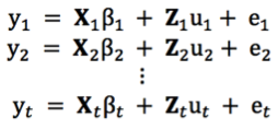
where y_i is a vector of trait phenotypes, \beta_i is a vector of fixed effects, u_i is a vector of random effects for individuals and e_i are residuals for trait i (i = 1,..., t). The random effects (u_1 ... u_i and e_i) are assumed to be normally distributed with mean zero. X and Z are incidence matrices for fixed and random effects respectively. The distribution of the multivariate response and the phenotypic variance covariance (V) are:

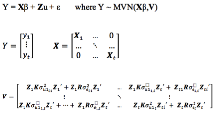
where K is the relationship or covariance matrix for the kth random effect (u=1,...,k), and R=I is an identity matrix for the residual term. The terms \sigma^2_{g_{i}} and \sigma^2_{\epsilon_{i}} denote the genetic (or any of the kth random terms) and residual variance of trait i, respectively and \sigma_{g_{_{ij}}} and \sigma_{\epsilon_{_{ij}}} the genetic (or any of the kth random terms) and residual covariance between traits i and j (i=1,...,t, and j=1,...,t). The algorithm implemented optimizes the log likelihood:

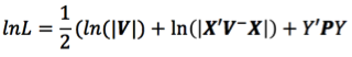
where || is the determinant of a matrix. And the REML estimates are updated using a Newton optimization algorithm of the form:

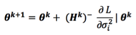
Where, theta is the vector of variance components for random effects and covariance components among traits, H^-1 is the inverse of the Hessian matrix of second derivatives for the kth cycle, dL/dsigma^2_i is the vector of first derivatives of the likelihood with respect to the variance-covariance components. The Eigen decomposition of the relationship matrix proposed by Lee and Van Der Werf (2016) was included in the Newton-Raphson algorithm to improve time efficiency. Additionally, the popular vpredict function to estimate standard errors for linear combinations of variance components (i.e. heritabilities and genetic correlations) was added to the package as well.

Bug report and contact

If you have any questions or suggestions please post it in https://stackoverflow.com or https://stats.stackexchange.com

I'll be glad to help or answer any question. I have spent a valuable amount of time developing this package. Please cite this package in your publication. Type 'citation("sommer")' to know how to cite it.

Author(s)

Giovanny Covarrubias-Pazaran

References

Covarrubias-Pazaran G. 2016. Genome assisted prediction of quantitative traits using the R package sommer. PLoS ONE 11(6): doi:10.1371/journal.pone.0156744

Covarrubias-Pazaran G. 2018. Software update: Moving the R package sommer to multivariate mixed models for genome-assisted prediction. doi: https://doi.org/10.1101/354639

Sanderson, C., & Curtin, R. (2025). Armadillo: An Efficient Framework for Numerical Linear Algebra. arXiv preprint arXiv:2502.03000.

Bernardo Rex. 2010. Breeding for quantitative traits in plants. Second edition. Stemma Press. 390 pp.

Gilmour et al. 1995. Average Information REML: An efficient algorithm for variance parameter estimation in linear mixed models. Biometrics 51(4):1440-1450.

Henderson C.R. 1975. Best Linear Unbiased Estimation and Prediction under a Selection Model. Biometrics vol. 31(2):423-447.

Kang et al. 2008. Efficient control of population structure in model organism association mapping. Genetics 178:1709-1723.

Lee et al. 2015. MTG2: An efficient algorithm for multivariate linear mixed model analysis based on genomic information. Cold Spring Harbor. doi: http://dx.doi.org/10.1101/027201.

Maier et al. 2015. Joint analysis of psychiatric disorders increases accuracy of risk prediction for schizophrenia, bipolar disorder, and major depressive disorder. Am J Hum Genet; 96(2):283-294.

Searle. 1993. Applying the EM algorithm to calculating ML and REML estimates of variance components. Paper invited for the 1993 American Statistical Association Meeting, San Francisco.

Yu et al. 2006. A unified mixed-model method for association mapping that accounts for multiple levels of relatedness. Genetics 38:203-208.

Tunnicliffe W. 1989. On the use of marginal likelihood in time series model estimation. JRSS 51(1):15-27.

Examples

####=========================================####
#### For CRAN time limitations most lines in the 
#### examples are silenced with one '#' mark, 
#### remove them and run the examples
####=========================================####

####=========================================####
#### EXAMPLES
#### Different models with sommer
####=========================================####

data(DT_example)

# DT <- DT_example
# DT=DT[with(DT, order(Env)), ]
# head(DT)
# 
# ####=========================================####
# #### Univariate homogeneous variance models  ####
# ####=========================================####
# 
# ## Compound simmetry (CS) model
# ans1 <- mmes(Yield~Env,
#              random= ~ Name + Env:Name,
#              rcov= ~ units,
#              data=DT)
# summary(ans1)
# 
# ####===========================================####
# #### Univariate heterogeneous variance models  ####
# ####===========================================####
# ## Compound simmetry (CS) + Diagonal (DIAG) model
# ans3 <- mmes(Yield~Env,
#              random= ~Name + vsm(dsm(Env),ism(Name)),
#              rcov= ~ vsm(dsm(Env),ism(units)),
#              data=DT)
# summary(ans3)

Two-dimensional penalised tensor-product of marginal B-Spline basis.

Description

Auxiliary function used for modelling the spatial or environmental effect as a two-dimensional penalised tensor-product (isotropic approach) based on Lee et al. (2013) and Rodriguez-Alvarez et al. (2018). This is a modified wrapper of some portions of the SpATS package to build a single incidence matrix containing all the columns from tensor products of the x and y coordinates and it fits such matrix as a single random effect. Then the heterogeneous covariances structure capabilities of sommer can be used to enhance the model fit. You may be interested in reading and citing not only sommec but also Wageningen publications if using this 2D spline methodology.

Usage

spl2Dc(x.coord,y.coord,at.var=NULL,at.levels=NULL, type="PSANOVA", 
      nsegments = c(10,10), penaltyord = c(2,2), degree = c(3,3), 
      nestorder = c(1,1), thetaC=NULL, theta=NULL, sp=FALSE)

Arguments

Details

The following documentation is taken from the SpATS package. Please refer to this package and associated publications if you are interested in going deeper on this technique:

Within the P-spline framework, anisotropic low-rank tensor-product smoothers have become the general approach for modelling multidimensional surfaces (Eilers and Marx 2003; Wood 2006). In the original SpATS package, was proposed to model the spatial or environmental effect by means of the tensor-product of B-splines basis functions. In other words, was proposed to model the spatial trend as a smooth bivariate surface jointly defined over the the spatial coordinates. Accordingly, the current function has been designed to allow the user to specify the spatial coordinates that the spatial trend is a function of. There is no restriction about how the spatial coordinates shall be specified: these can be the longitude and latitude of the position of the plot on the field or the column and row numbers. The only restriction is that the variables defining the spatial coordinates should be numeric (in contrast to factors).

As far as estimation is concerned, we have used in this package the equivalence between P-splines and linear mixed models (Currie and Durban, 2002). Under this approach, the smoothing parameters are expressed as the ratio between variance components. Moreover, the smooth components are decomposed in two parts: one which is not penalised (and treated as fixed) and one with is penalised (and treated as random). For the two-dimensional case, the mixed model representation leads also to a very interesting decomposition of the penalised part of the bivariate surface in three different components (Lee and Durban, 2011): (a) a component that contains the smooth main effect (smooth trend) along one of the covariates that the surface is a function of (as, e.g, the x-spatial coordinate or column position of the plot in the field), (b) a component that contains the smooth main effect (smooth trend) along the other covariate (i.e., the y-spatial coordinate or row position); and (c) a smooth interaction component (sum of the linear-by-smooth interaction components and the smooth-by-smooth interaction component).

The original implementation of SpATS assumes two different smoothing parameters, i.e., one for each covariate in the smooth component. Accordingly, the same smoothing parameters are used for both, the main effects and the smooth interaction. However, this approach can be extended to deal with the ANOVA-type decomposition presented in Lee and Durban (2011). In their approach, four different smoothing parameters are considered for the smooth surface, that are in concordance with the aforementioned decomposition: (a) two smoothing parameter, one for each of the main effects; and (b) two smoothing parameter for the smooth interaction component.

It should be noted that, the computational burden associated with the estimation of the two-dimensional tensor-product smoother might be prohibitive if the dimension of the marginal bases is large. In these cases, Lee et al. (2013) propose to reduce the computational cost by using nested bases. The idea is to reduce the dimension of the marginal bases (and therefore the associated number of parameters to be estimated), but only for the smooth-by-smooth interaction component. As pointed out by the authors, this simplification can be justified by the fact that the main effects would in fact explain most of the structure (or spatial trend) presented in the data, and so a less rich representation of the smooth-by-smooth interaction component could be needed. In order to ensure that the reduced bivariate surface is in fact nested to the model including only the main effects, Lee et al. (2013) show that the number of segments used for the nested basis should be a divisor of the number of segments used in the original basis (nsegments argument). In the present function, the divisor of the number of segments is specified through the argument nestorder. For a more detailed review on this topic, see Lee (2010) and Lee et al. (2013). The "PSANOVA" approach represents an alternative method. In this case, the smooth bivariate surface (or spatial trend) is decomposed in five different components each of them depending on a single smoothing parameter (see Lee et al., 2013).

—————–

As mentioned at the beginning, the piece of documentation stated above was taken completely from the SpATS package in order to provide a deeper explanation. In practice, sommec uses some pieces of code from SpATS to build the design matrix containing all the columns from tensor products of the x and y coordinates and it fits such matrix as a single random effect. As a result the same variance component is assumed for the linear, linear by linear, linear by spline, and spline by spline interactions. This results in a less flexible approach than the one proposed by Rodriguez-Alvarez et al. (2018) but still makes a pretty good job to model the spatial variation. Use under your own risk.

References

Rodriguez-Alvarez, M.X, Boer, M.P., van Eeuwijk, F.A., and Eilers, P.H.C. (2018). SpATS: Spatial Analysis of Field Trials with Splines. R package version 1.0-9. https://CRAN.R-project.org/package=SpATS.

Rodriguez-Alvarez, M.X., et al. (2015) Fast smoothng parameter separaton n multdmensonal generalzed P-splnes: the SAP algorthm. Statistics and Computing 25.5: 941-957.

Lee, D.-J., Durban, M., and Eilers, P.H.C. (2013). Efficient two-dimensional smoothing with P-spline ANOVA mixed models and nested bases. Computational Statistics and Data Analysis, 61, 22 - 37.

Gilmour, A.R., Cullis, B.R., and Verbyla, A.P. (1997). Accounting for Natural and Extraneous Variation in the Analysis of Field Experiments. Journal of Agricultural, Biological, and Environmental Statistics, 2, 269 - 293.

See Also

mmes

Examples

## ============================ ##
## example to use spl2Dc() 
## ============================ ## 
data(DT_cpdata)
# DT <- DT_cpdata
# GT <- GT_cpdata
# MP <- MP_cpdata
# A <- A.mat(GT)
## ============================ ##
## mimic 2 fields
## ============================ ## 
# aa <- DT; bb <- DT
# aa$FIELD <- "A";bb$FIELD <- "B"
# set.seed(1234)
# aa$Yield <- aa$Yield + rnorm(length(aa$Yield),0,4)
# DT2 <- rbind(aa,bb)
# head(DT2)
# mix <- mmes(Yield~1, henderson = F,
#             random=~
#               vsm(dsm(FIELD),ism(Rowf)) +
#               vsm(dsm(FIELD),ism(Colf)) +
#                 spl2Dc(Row,Col,at.var=FIELD),
#             rcov=~vsm(dsm(FIELD),ism(units)),
#             data=DT2)
# 
# # extract spatial effects
# blup <- mix$uList$`spl2Dc(Row, Col, at.var = FIELD`
# head(blup) # 2 fields
# # recreate the incidence matrices
# xx=with(DT2, spl2Dc(Row,Col,at.var=FIELD))
# # get fitted values Zu for spatial effects and add them to the dataset
# field1 <- xx$Z$`A:all` %*% blup[,1]
# field2 <- xx$Z$`B:all` %*% blup[,2]
# DT2$spat <- field1+field2
# # plots the spatial effects
# lattice::levelplot(spat~Row*Col|FIELD, data=DT2)

Get Tensor Product Spline Mixed Model Incidence Matrices

Description

spl2Dmats gets Tensor-Product P-Spline Mixed Model Incidence Matrices for use with sommer and its main function mmes. We thank Sue Welham for making the TPSbits package available to the community. If you're using this function for your research please cite her TPSbits package :) this is mostly a wrapper of her tpsmmb function to enable the use in sommer.

Usage

spl2Dmats(
  x.coord.name,
  y.coord.name,
  data,
  at.name,
  at.levels, 
  nsegments=NULL,
  minbound=NULL,
  maxbound=NULL,
  degree = c(3, 3),
  penaltyord = c(2,2), 
  nestorder = c(1,1),
  method = "Lee"
)

Arguments

Value

List of length 7 elements:

1. data = the input data frame augmented with structures required to fit tensor product splines in asreml-R. This data frame can be used to fit the TPS model.

   Added columns:

   • TP.col, TP.row = column and row coordinates

   • TP.CxR = combined index for use with smooth x smooth term

   • TP.C.n for n=1:(diff.c) = X parts of column spline for use in random model (where diff.c is the order of column differencing)

   • TP.R.n for n=1:(diff.r) = X parts of row spline for use in random model (where diff.r is the order of row differencing)

   • TP.CR.n for n=1:((diff.c*diff.r)) = interaction between the two X parts for use in fixed model. The first variate is a constant term which should be omitted from the model when the constant (1) is present. If all elements are included in the model then the constant term should be omitted, eg. y ~ -1 + TP.CR.1 + TP.CR.2 + TP.CR.3 + TP.CR.4 + other terms...

   • when asreml="grp" or "sepgrp", the spline basis functions are also added into the data frame. Column numbers for each term are given in the grp list structure.

2. fR = Xr1:Zc

3. fC = Xr2:Zc

4. fR.C = Zr:Xc1

5. R.fC = Zr:Xc2

6. fR.fC = Zc:Zr

7. all = Xr1:Zc | Xr2:Zc | Zr:Xc1 | Zr:Xc2 | Zc:Zr

Examples

data("DT_cpdata")
DT <- DT_cpdata
GT <- GT_cpdata
MP <- MP_cpdata
#### create the variance-covariance matrix
A <- A.mat(GT) # additive relationship matrix

M <- spl2Dmats(x.coord.name = "Col", y.coord.name = "Row", data=DT, nseg =c(14,21))
head(M$data)
# m1g <- mmes(Yield~1+TP.CR.2+TP.CR.3+TP.CR.4,
#             random=~Rowf+Colf+vsm(ism(M$fC))+vsm(ism(M$fR))+
#               vsm(ism(M$fC.R))+vsm(ism(M$C.fR))+vsm(ism(M$fC.fR))+
#               vsm(ism(id),Gu=A),
#             data=M$data, tolpar = 1e-6,
#             iters=30)
# 
# summary(m1g)$varcomp

Stacking traits in a dataset

Description

stackTrait creates a dataset stacking traits in the long format to be used with the mmes solver for multi-trait models.

Usage

  stackTrait(data, traits)

Arguments

Value

$res

a data frame with traits in long format.

Author(s)

Giovanny Covarrubias-Pazaran

References

Covarrubias-Pazaran G (2016) Genome assisted prediction of quantitative traits using the R package sommer. PLoS ONE 11(6): doi:10.1371/journal.pone.0156744

Examples

data(DT_example)
DT <- DT_example
A <- A_example
head(DT)

DT2 <- stackTrait(DT, traits = c("Yield","Weight"))
head(DT2)

Standardize a vector of values in range 0 to 1

Description

Simple function to map a vector of values to the range of 0 and 1 values to have a better behavior of the algorithm.

Usage

stan(x, lb=0, ub=1)

Arguments

Details

Simple function to map a vector of values to the range of 0 and 1 values to have a better behavior of the algorithm.

Value

$res

new values in range 0 to 1

References

Covarrubias-Pazaran G (2016) Genome assisted prediction of quantitative traits using the R package sommer. PLoS ONE 11(6): doi:10.1371/journal.pone.0156744

Examples

x <- rnorm(20, 10, 3);x
stan(x)

summary form a GLMM fitted with mmer

Description

summary method for class "mmer".

Usage

## S3 method for class 'mmer'
summary(object, ...)

Arguments

Value

vector of summary

Author(s)

Giovanny Covarrubias-Pazaran

See Also

summary, mmer

summary form a GLMM fitted with mmes

Description

summary method for class "mmes".

Usage

## S3 method for class 'mmes'
summary(object, ...)

Arguments

Value

vector of summary

Author(s)

Giovanny Covarrubias-Pazaran

See Also

summary, mmes

Get Tensor Product Spline Mixed Model Incidence Matrices

Description

tps is a wrapper of tpsmmb function from the TPSbits package to avoid version dependencies but if you're using this function for your research please cite the TPSbits package. This function is internally used by the spl2Dmatrices function to get Tensor-Product P-Spline Mixed Model Bits (design matrices) for use with sommer.

Usage

tps(
  columncoordinates,
  rowcoordinates,
  nsegments=NULL,
  minbound=NULL,
  maxbound=NULL,
  degree = c(3, 3),
  penaltyord = c(2, 2),
  nestorder = c(1, 1),
  asreml = "grp",
  eigenvalues = "include",
  method = "Lee",
  stub = NULL
)

Arguments

Value

List of length 7, 8 or 9 (according to the asreml and eigenvalues parameter settings).

1. data = the input data frame augmented with structures required to fit tensor product splines in asreml-R. This data frame can be used to fit the TPS model.

   Added columns:

   • TP.col, TP.row = column and row coordinates

   • TP.CxR = combined index for use with smooth x smooth term

   • TP.C.n for n=1:(diff.c) = X parts of column spline for use in random model (where diff.c is the order of column differencing)

   • TP.R.n for n=1:(diff.r) = X parts of row spline for use in random model (where diff.r is the order of row differencing)

   • TP.CR.n for n=1:((diff.c*diff.r)) = interaction between the two X parts for use in fixed model. The first variate is a constant term which should be omitted from the model when the constant (1) is present. If all elements are included in the model then the constant term should be omitted, eg. y ~ -1 + TP.CR.1 + TP.CR.2 + TP.CR.3 + TP.CR.4 + other terms...

   • when asreml="grp" or "sepgrp", the spline basis functions are also added into the data frame. Column numbers for each term are given in the grp list structure.

2. mbflist = list that can be used in call to asreml (so long as Z matrix data frames extracted with right names, eg BcZ<stub>.df)

3. BcZ.df = mbf data frame mapping onto smooth part of column spline, last column (labelled TP.col) gives column index

4. BrZ.df = mbf data frame mapping onto smooth part of row spline, last column (labelled TP.row) gives row index

5. BcrZ.df = mbf data frame mapping onto smooth x smooth term, last column (labelled TP.CxR) maps onto col x row combined index

6. dim = list structure, holding dimension values relating to the model:

   1. "diff.c" = order of differencing used in column dimension

   2. "nbc" = number of random basis functions in column dimension

   3. "nbcn" = number of nested random basis functions in column dimension used in smooth x smooth term

   4. "diff.r" = order of differencing used in column dimension

   5. "nbr" = number of random basis functions in column dimension

   6. "nbrn" = number of nested random basis functions in column dimension used in smooth x smooth term

7. trace = list of trace values for ZGZ' for the random TPspline terms, where Z is the design matrix and G is the known diagonal variance matrix derived from eigenvalues. This can be used to rescale the spline design matrix (or equivalently variance components).

8. grp = list structure, only added for settings asreml="grp", asreml="sepgrp" or asreml="own". For asreml="grp", provides column indexes for each of the 5 random components of the 2D splines. For asreml="sepgrp", provides column indexes for each of the X and Z component matrices for the 1D splines, plus the composite smooth x smooth interaction term. For asreml="own", provides column indexes for the composite random model. Dimensions of the components can be derived from the values in the dim item. The Z terms are scaled by the associated eigenvalues when eigenvalues="include", but not when eigenvalues="omit".

9. eigen = list structure, only added for option setting eigenvalues="omit". Holds the diagonal elements of the inverse variance matrix for the terms Xc:Zr (called diagr), Zc:Xr (called diagc) and Zc:Zr (called diagcr).

Get Tensor Product Spline Mixed Model Incidence Matrices

Description

tpsmmbwrapper is a wrapper of tpsmmb function from the TPSbits package to avoid version dependencies but if you're using this function for your research please cite the TPSbits package. This function is internally used by the spl2Dmatrices function to get Tensor-Product P-Spline Mixed Model Bits (design matrices) for use with sommer.

Usage

tpsmmbwrapper(
  columncoordinates,
  rowcoordinates,
  data,
  nsegments=NULL,
  minbound=NULL,
  maxbound=NULL,
  degree = c(3, 3),
  penaltyord = c(2, 2),
  nestorder = c(1, 1),
  asreml = "mbf",
  eigenvalues = "include",
  method = "Lee",
  stub = NULL
)

Arguments

Value

List of length 7, 8 or 9 (according to the asreml and eigenvalues parameter settings).

1. data = the input data frame augmented with structures required to fit tensor product splines in asreml-R. This data frame can be used to fit the TPS model.

   Added columns:

   • TP.col, TP.row = column and row coordinates

   • TP.CxR = combined index for use with smooth x smooth term

   • TP.C.n for n=1:(diff.c) = X parts of column spline for use in random model (where diff.c is the order of column differencing)

   • TP.R.n for n=1:(diff.r) = X parts of row spline for use in random model (where diff.r is the order of row differencing)

   • TP.CR.n for n=1:((diff.c*diff.r)) = interaction between the two X parts for use in fixed model. The first variate is a constant term which should be omitted from the model when the constant (1) is present. If all elements are included in the model then the constant term should be omitted, eg. y ~ -1 + TP.CR.1 + TP.CR.2 + TP.CR.3 + TP.CR.4 + other terms...

   • when asreml="grp" or "sepgrp", the spline basis functions are also added into the data frame. Column numbers for each term are given in the grp list structure.

2. mbflist = list that can be used in call to asreml (so long as Z matrix data frames extracted with right names, eg BcZ<stub>.df)

3. BcZ.df = mbf data frame mapping onto smooth part of column spline, last column (labelled TP.col) gives column index

4. BrZ.df = mbf data frame mapping onto smooth part of row spline, last column (labelled TP.row) gives row index

5. BcrZ.df = mbf data frame mapping onto smooth x smooth term, last column (labelled TP.CxR) maps onto col x row combined index

6. dim = list structure, holding dimension values relating to the model:

   1. "diff.c" = order of differencing used in column dimension

   2. "nbc" = number of random basis functions in column dimension

   3. "nbcn" = number of nested random basis functions in column dimension used in smooth x smooth term

   4. "diff.r" = order of differencing used in column dimension

   5. "nbr" = number of random basis functions in column dimension

   6. "nbrn" = number of nested random basis functions in column dimension used in smooth x smooth term

7. trace = list of trace values for ZGZ' for the random TPspline terms, where Z is the design matrix and G is the known diagonal variance matrix derived from eigenvalues. This can be used to rescale the spline design matrix (or equivalently variance components).

8. grp = list structure, only added for settings asreml="grp", asreml="sepgrp" or asreml="own". For asreml="grp", provides column indexes for each of the 5 random components of the 2D splines. For asreml="sepgrp", provides column indexes for each of the X and Z component matrices for the 1D splines, plus the composite smooth x smooth interaction term. For asreml="own", provides column indexes for the composite random model. Dimensions of the components can be derived from the values in the dim item. The Z terms are scaled by the associated eigenvalues when eigenvalues="include", but not when eigenvalues="omit".

9. eigen = list structure, only added for option setting eigenvalues="omit". Holds the diagonal elements of the inverse variance matrix for the terms Xc:Zr (called diagr), Zc:Xr (called diagc) and Zc:Zr (called diagcr).

Creating color with transparency

Description

This function takes a color and returns the same with a certain alpha grade transparency.

Usage

transp(col, alpha=0.5)

Arguments

Details

No major details.

Value

If arguments are correctly specified the function returns:

$res

A new color with certain grade of transparency

References

Robert J. Henry. 2013. Molecular Markers in Plants. Wiley-Blackwell. ISBN 978-0-470-95951-0.

Ben Hui Liu. 1998. Statistical Genomics. CRC Press LLC. ISBN 0-8493-3166-8.

Examples

transp("red", alpha=0.5)

unstructured indication matrix

Description

unsm creates a square matrix with ones in the diagonals and 2's in the off-diagonals to quickly specify an unstructured constraint in the Gtc argument of the vsm function.

Usage

  unsm(x, reps=NULL)

Arguments

Value

$res

a matrix or a list of matrices with the constraints to be provided in the Gtc argument of the vsm function.

Author(s)

Giovanny Covarrubias-Pazaran

References

Covarrubias-Pazaran G (2016) Genome assisted prediction of quantitative traits using the R package sommer. PLoS ONE 11(6): doi:10.1371/journal.pone.0156744

Examples

unsm(3)
unsm(3,2)

unstructured covariance structure

Description

usm creates an unstructured covariance structure for specific levels of the random effect to be used with the mmes solver.

Usage

  usm(x, thetaC, theta)

Arguments

Value

$res

a list with the provided vector and the variance covariance structure expected for the levels of the random effect.

Author(s)

Giovanny Covarrubias-Pazaran

References

Covarrubias-Pazaran G (2016) Genome assisted prediction of quantitative traits using the R package sommer. PLoS ONE 11(6): doi:10.1371/journal.pone.0156744

Examples

x <- as.factor(c(1:5,1:5,1:5));x
usm(x)
## how to use the theta and thetaC arguments:
# data(DT_example)
# DT <- DT_example
# theta <- matrix(9:1,3,3); 
# theta[lower.tri(theta)] <- t(theta)[lower.tri(theta)] 
# theta # initial VCs
# thetaC <- fixm(3); thetaC # fixed VCs
# ans1 <- mmes(Yield~Env,
#              random= ~ vsm( usm(Env,theta = theta,thetaC = thetaC),ism(Name) ),
#              rcov= ~ units, nIters = 1,
#              data=DT)
# summary(ans1)$varcomp

vpredict form of a LMM fitted with mmes

Description

vpredict method for class "mmes".

Post-analysis procedure to calculate linear combinations of variance components. Its intended use is when the variance components are either simple variances or are variances and covariances in an unstructured matrix. The functions covered are linear combinations of the variance components (for example, phenotypic variance), a ratio of two components (for example, heritabilities) and the correlation based on three components (for example, genetic correlation).

The calculations are based on the estimated variance parameters and their variance matrix as represented by the inverse of the Fisher or Average information matrix. Note that this matrix has zero values for fixed variance parameters including those near the parameter space boundary.

The transform is specified with a formula. On the left side of the formula is a name for the transformation. On the right side of the formula is a transformation specified with shortcut names like 'V1', 'V2', etc. The easiest way to identify these shortcut names is to use 'summary(object)$varcomp'. The rows of this object can referred to with shortcuts 'V1', 'V2', etc. See the example below.

Usage

vpredict(object, transform)
## S3 method for class 'mmes'
vpredict(object, transform)

Arguments

Details

The delta method (e.g., Lynch and Walsh 1998, Appendix 1; Ver Hoef 2012) uses a Taylor series expansion to approximate the moments of a function of parameters. Here, a second-order Taylor series expansion is implemented to approximate the standard error for a function of (co)variance parameters. Partial first derivatives of the function are calculated by algorithmic differentiation with deriv.

Though vpredict can calculate standard errors for non-linear functions of (co)variance parameters from a fitted mmes model, it is limited to non-linear functions constructed by mathematical operations such as the arithmetic operators +, -, *, / and ^, and single-variable functions such as exp and log. See deriv for more information.

Value

Author(s)

Giovanny Covarrubias

References

Covarrubias-Pazaran G (2016) Genome assisted prediction of quantitative traits using the R package sommer. PLoS ONE 11(6): doi:10.1371/journal.pone.0156744

Lynch, M. and B. Walsh 1998. Genetics and Analysis of Quantitative Traits. Sinauer Associates, Inc., Sunderland, MA, USA.

Ver Hoef, J.M. 2012. Who invented the delta method? The American Statistician 66:124-127. DOI: 10.1080/00031305.2012.687494

See Also

vpredict, mmes

Examples

####=========================================####
####=========================================####
#### EXAMPLE 1
#### simple example with univariate models
####=========================================####
####=========================================####
# data(DT_cpdata)
# DT <- DT_cpdata
# GT <- GT_cpdata
# MP <- MP_cpdata
# #### create the variance-covariance matrix 
# A <- A.mat(GT)
# #### look at the data and fit the model
# head(DT)
# mix1 <- mmes(Yield~1,
#               random=~vsm(ism(id),Gu=A), 
#               data=DT)
# summary(mix1)$varcomp
# #### run the vpredict function
# vpredict(mix1, h2 ~ V1 / ( V1 + V2 ) )

variance structure specification

Description

vs DEPRECATED NOW. was the main function to build the variance-covariance structure for the random effects to be fitted in the mmer solver.

Usage

  vs(..., Gu=NULL, Gti=NULL, Gtc=NULL, reorderGu=TRUE, buildGu=TRUE)

Arguments

Details

When providing initial values in the Gti argument the user has to provide scaled variance component values. The user can provide values from a previous model by accessing the sigma_scaled output from an mmer model or if an specific value is desired the user can obtain the scaled value as:

m = x/var(y)

where x is the desired initial value and y is the response variable. You can find an example in the DT_cpdata dataset.

Value

$res

a list with all neccesary elements (incidence matrices, known var-cov structures, unknown covariance structures to be estimated and constraints) to be used in the mmer solver.

Author(s)

Giovanny Covarrubias-Pazaran

References

Covarrubias-Pazaran G (2016) Genome assisted prediction of quantitative traits using the R package sommer. PLoS ONE 11(6): doi:10.1371/journal.pone.0156744

Covarrubias-Pazaran G (2018) Software update: Moving the R package sommer to multivariate mixed models for genome-assisted prediction. doi: https://doi.org/10.1101/354639

See Also

The core function of the package: mmer

Examples

data(DT_example)
DT <- DT_example
A <- A_example

## ============================ ##
## example to without structure
## ============================ ##

mix <- mmer(Yield~Env, 
            random= ~ vs(Name),
            rcov=~ vs(units),
            data=DT)

variance structure specification

Description

vsm is the main function to build the variance-covariance structure for the random effects to be fitted in the mmes solver.

Usage

  vsm(..., Gu=NULL, buildGu=TRUE, meN=1, meTheta=NULL, meThetaC=NULL, 
      sp=FALSE, isFixed=FALSE, verbose=TRUE)

Arguments

Details

...

Value

$res

a list with all neccesary elements (incidence matrices, known var-cov structures, unknown covariance structures to be estimated and constraints) to be used in the mmes solver.

Author(s)

Giovanny Covarrubias-Pazaran

References

Covarrubias-Pazaran G (2016) Genome assisted prediction of quantitative traits using the R package sommer. PLoS ONE 11(6): doi:10.1371/journal.pone.0156744

Covarrubias-Pazaran G (2018) Software update: Moving the R package sommer to multivariate mixed models for genome-assisted prediction. doi: https://doi.org/10.1101/354639

See Also

The core function of the package: mmes

Examples

data(DT_example)
DT <- DT_example
DT=DT[with(DT, order(Env)), ]
A <- A_example

# if using mmes=TRUE remember to provide relationship as inverse in the Gu argument
# Ai <- solve(A + diag(1e-4,ncol(A),ncol(A)))
# Ai <- as(as(as( Ai,  "dMatrix"), "generalMatrix"), "CsparseMatrix")

x <- as.character(unique(DT$Name))
DT <- droplevels(DT[which(!is.na(match(DT$Name, x[1:5]))),])
## ============================ ##
## example without structure
## ============================ ##
ism(DT$Name)
mix <- mmes(Yield~Env,
            random= ~ vsm(ism(Name)),
            rcov=~ units,
            nIters=10,
            data=DT)

## ============================ ##
## example to without structure but
## using covariance among levels in the
## random effect Name
## ============================ ##
mix <- mmes(Yield~Env, 
            random= ~ vsm(ism(Name), Gu=A),
            rcov=~ units,
            nIters=10,
            data=DT)
summary(mix)$varcomp
## ============================ ##
## example to use dsm() structure (DIAGONAL)
## ============================ ##
dsm(DT$Year)
mix <- mmes(Yield~Env,
            random= ~ vsm(dsm(Year),ism(Name)),
            rcov=~ vsm(dsm(Year),ism(units)),
            nIters=10,
            data=DT)
summary(mix)$varcomp
## ============================ ##
## example to use atm() structure (level-specific)
## ============================ ##
# unique(DT$Year)
# mix <- mmes(Yield~Env,
#             random= ~ vsm(atm(Year,c("2011","2012")),ism(Name)),
#             rcov=~ vsm(dsm(Year),ism(units)),
#             data=DT)
## ============================ ##
## example to use usm() structure (UNSTRUCTURED)
## ============================ ##
usm(DT$Year)
mix <- mmes(Yield~Env,
            random= ~ vsm(usm(Year),ism(Name)),
            rcov=~ vsm(dsm(Year),ism(units)),
            nIters = 10,
            data=DT)
## ============================ ##
## example using structure in fixed effect
## (notice the isFixed argument)
## ============================ ##
mix <- mmes(Yield~ vsm(atm(Env,"CA.2011"), ism(Name), isFixed = TRUE),
            rcov=~ units,
            nIters=10,
            data=DT)

variance structure specification

Description

vsr DEPRECATED NOW. was the main function to build the variance-covariance structure for the random effects to be fitted in the mmer solver.

Usage

  vsr(..., Gu=NULL, Gti=NULL, Gtc=NULL, reorderGu=TRUE, buildGu=TRUE)

Arguments

Details

When providing initial values in the Gti argument the user has to provide scaled variance component values. The user can provide values from a previous model by accessing the sigma_scaled output from an mmer model or if an specific value is desired the user can obtain the scaled value as:

m = x/var(y)

where x is the desired initial value and y is the response variable. You can find an example in the DT_cpdata dataset.

Value

$res

a list with all neccesary elements (incidence matrices, known var-cov structures, unknown covariance structures to be estimated and constraints) to be used in the mmer solver.

Author(s)

Giovanny Covarrubias-Pazaran

References

Covarrubias-Pazaran G (2016) Genome assisted prediction of quantitative traits using the R package sommer. PLoS ONE 11(6): doi:10.1371/journal.pone.0156744

Covarrubias-Pazaran G (2018) Software update: Moving the R package sommer to multivariate mixed models for genome-assisted prediction. doi: https://doi.org/10.1101/354639

Examples

data(DT_example)
DT <- DT_example
A <- A_example

## ============================ ##
## example to without structure
## ============================ ##

mix <- mmer(Yield~Env, 
            random= ~ vsr(Name),
            rcov=~ vsr(units),
            data=DT)

Wald Test for Model Coefficients

Description

Computes a Wald \chi^2 test for 1 or more coefficients, given their variance-covariance matrix.

Usage

  wald.test(Sigma, b, Terms = NULL, L = NULL, H0 = NULL,  
            df = NULL, verbose = FALSE)
  ## S3 method for class 'wald.test'
print(x, digits = 2, ...)
  

Arguments

Details

The key assumption is that the coefficients asymptotically follow a (multivariate) normal distribution with mean = model coefficients and variance = their var-cov matrix.
One (and only one) of Terms or L must be given. When L is given, it must have the same number of columns as the length of b, and the same number of rows as the number of linear combinations of coefficients. When df is given, the \chi^2 Wald statistic is divided by m = the number of linear combinations of coefficients to be tested (i.e., length(Terms) or nrow(L)). Under the null hypothesis H0, this new statistic follows an F(m, df) distribution.

Value

An object of class wald.test, printed with print.wald.test.

References

Diggle, P.J., Liang, K.-Y., Zeger, S.L., 1994. Analysis of longitudinal data. Oxford, Clarendon Press, 253 p.
Draper, N.R., Smith, H., 1998. Applied Regression Analysis. New York, John Wiley & Sons, Inc., 706 p.

Examples

data(DT_yatesoats)
DT <- DT_yatesoats

m3 <- mmes(fixed=Y ~ V + N + V:N-1,
           random = ~ B + B:MP,
           rcov=~units,
           data = DT)

wald.test(b = m3$b, Sigma = m3$Ci[1:nrow(m3$b),1:nrow(m3$b)], Terms = 2)

LL <- matrix(0,nrow=1, ncol=12)
LL[1,2] <- 1
LL[1,3] <- -1
LL

wald.test(b = m3$b, Sigma = m3$Ci[1:nrow(m3$b),1:nrow(m3$b)], L=LL)