





This package contains functions to compute, visualize and compare Least Squares Sparse Principal Components Analysis (LS-SPCA). Differently from other conventional SPCA methods, LS-SPCA provides a close approximation to the PCs, thus something like PCA with sparse weights.
An efficient C++ backend makes the fitting functions
fast and memory efficient. Careful input validation and error handling
prevents crashes and provides useful error and warning messages.
Methodological details, references and full presentation can be found in the spca_extended vignette.
The stable release version can be installed from CRAN
install.packages("spca")The current development version can be installed from GitHub with
remotes::install_github("merolagio/spca")The main function spca() computes the sparse weights and
various statistics, such as the variance explained by each sparse
component (sPC). In a typical LS-SPCA workflow, the number of sPCs to
compute is chosen by examining visually the eigenvalues of the
covariance/correlation matrix. These can be computed and stored in a
compatible object of class (pca, spca) with the function
pca().
Different methods can be applied to class spca objects:
additionally to standard print(), summary()
and plot(), also aggregate_by_group() (to
visualize the contribution by scale), change_sign() and
show_weights() and show_correlations() are
available.
The function compare_spca() compares two or more
spca solutions, aggregate_by_group()
summarizes weights or contributions by group, and
new_spca() creates an spca object from a set
of weights. Additional methods include show_weights(),
which displays nonzero weights or contributions;
show_correlations(), which displays correlations among sPCs
and between sPCs and the corresponding PCs; and
change_sign(), which changes the signs of selected
components and their associated quantities. The functions
mp_qqplot() and scree_plot() produce
diagnostic plots from an object returned by pca().
The holzinger dataset is the small classic
Holzinger-Swineford dataset with 145 cases on 12 variables grouped in 4
scales.
library(spca)
data(holzinger)
dim(holzinger)
#> [1] 145  12
data(holzinger_scales)
holzinger_scales
#>  [1] SPL SPL SPL VBL VBL VBL SPD SPD SPD MTH MTH MTH
#> Levels: SPL VBL SPD MTHho_pca = pca(holzinger, screeplot = TRUE, qq_plot = TRUE)
summary(ho_pca, cols = 10)
#> PC1 PC2 PC3 PC4 PC5 PC6 PC7 PC8 PC9 PC10
#> Vexp 40.2% 13.7% 10.6% 6.4% 5.6% 5.1% 4.3% 3.9% 3.2% 2.6%
#> Cvexp 40.2% 53.9% 64.5% 70.9% 76.5% 81.6% 85.9% 89.8% 93.0% 95.6%
#> Card 12 12 12 12 12 12 12 12 12 12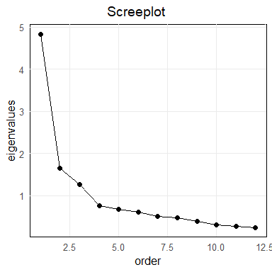
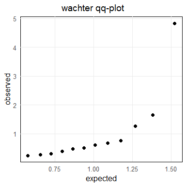
The screeplot would call for four components while the qqplot indicates three. We can settle for 4 components, ucknowledging that the fourth PC may be explaining mainly noise.
Important parameters in the spca() function are:
alpha which controls the minimum the minimum proportion
of ;objective sets which criterion is used to stop variable
selection: cumulative variance explained (RCVEXP) by the sPCs, relative
to that explained by the corresponding PCs [default], or \(`R^2`\) with the current PC;n_comps the number of components to compute;method the LS-SPCA method to use: “u” (for
uncorrelated), “c” (for correlated) [default]) or “p” (for
projection);var_selection which variable selection to use “forward”
[default], “stepwise”, or “backward”).See the spca help for details on these and more
parameters.
The following command computes four sPCs with
default settings: alpha = 0.95,
var_selection = forward, method = "c" that
selects the cSPCA method. Hence, we expect each sPC to
yield at least 95% cumulative VEXP, allowing some very mild correlation
between sPCs.
ho_spca = spca(holzinger, n_comps = 4)Methods are print, plot (several options
available) and summary. By defaut, plot and print show the
percentage contributions, that is the weights scaled to
have sum of their absolute values equal to 1.
ho_spca # print
#> Percentage contributions
#>             sPC1   sPC2   sPC3   sPC4
#> visual     11.9%                43.9%
#> cubes                    31.4% -21.3%
#> flags      14.2%         23.0%
#> paragraph        -21.6%
#> sentence   19.6%        -29.7%
#> wordm            -22.3%
#> addition   12.2%  27.5% -15.9% -10.6%
#> counting          28.6%
#> straight   12.3%
#> deduct     13.7%               -24.3%
#> series     16.1%
#>            -----  -----  -----  -----
#> Cvexp      38.6%  51.5%  61.4%  67.5%
#>

summary(ho_spca, cor_with_pc = TRUE)
#>         sPC1  sPC2  sPC3  sPC4
#> Vexp   38.6% 12.9%  9.9%  6.1%
#> Cvexp  38.6% 51.5% 61.4% 67.5%
#> Rvexp  96.0% 94.5% 93.5% 95.3%
#> Rcvexp 96.0% 95.6% 95.3% 95.3%
#> Card       7     4     4     4
#> r      0.978 0.946 0.925 0.762

plot(ho_spca, plot_type = "bar")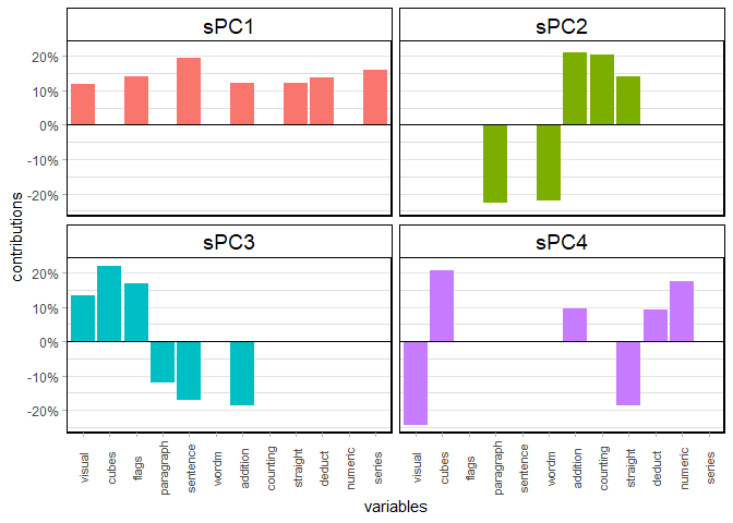
#sPCs correlation
show_correlations(ho_spca)
#>         sPC1  sPC2  sPC3  sPC4
#> sPC1    1.00 -0.01 -0.03 -0.02
#> sPC2   -0.01  1.00 -0.08 -0.10
#> sPC3   -0.03 -0.08  1.00 -0.06
#> sPC4   -0.02 -0.10 -0.06  1.00
#>        ----- ----- ----- -----
#> sPC-PC  0.98  0.95  0.92  0.76
the sparse weights can be compared to the full PCA weights with
compare_spca
compare_spca(list(ho_pca, ho_spca), variable_groups = holzinger_scales,
             x_axis_var_names = FALSE,  methods_names = c("PCA", "SPCA")
             )
#>        C1.M1  C1.M2  C2.M1  C2.M2  C3.M1  C3.M2  C4.M1  C4.M2
#> Vexp    40.2%  38.6%  13.7%  12.9%  10.6%   9.9%   6.4%   6.1%
#> Cvexp   40.2%  38.6%  53.9%  51.5%  64.5%  61.4%  70.9%  67.5%
#> Rvexp  100.0%  96.0% 100.0%  94.5% 100.0%  93.5% 100.0%  95.3%
#> Rcvexp 100.0%  96.0% 100.0%  95.6% 100.0%  95.3% 100.0%  95.3%
#> Card       12      7     12      4     12      4     12      4
#> abs_r    1.00   0.98   1.00   0.95   1.00   0.92   1.00   0.76
The variable_groups = group_factor adds lines separating
variable groups. Adding print_weights = TRUE would show the
contributions side by side.
Other plot types are available:
Circular:
plot(ho_spca, plot_type = "c") # "c" for "circular"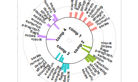
Heatmap:
plot(ho_spca, plot_type = "h", controls = list(legend_position = "b")) # "h" is enough to call "heatmap" type and "b" to indicate "bottom".
The variables in the holzinger dataset belong to four
different scales, recorded in the factor holzinger_scales.
These can be differentiated in the barplot
plot(ho_spca, plot_type = "bars", variable_groups = holzinger_scales, controls = list(legend_position = "right")) 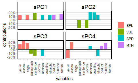
aggregate_by_group(ho_spca, variable_groups = holzinger_scales)
#>      sPC1   sPC2   sPC3   sPC4
#> SPL 26.0%         54.4%  22.6%
#> VBL 19.6% -43.9% -29.7%
#> SPD 24.6%  56.1% -15.9% -10.6%
#> MTH 29.8% -24.3%Compare the CSPCA solutions with alpha = 0.95 those with alpha = 0.90.
ho_spca90 = spca(holzinger, n_comps = 4, alpha = 0.9)

compare_spca(obj_list = list(ho_spca, ho_spca90),
             methods_names = c("alpha = 95", "alpha = 90"))
#>        C1.M1 C1.M2 C2.M1 C2.M2 C3.M1 C3.M2 C4.M1 C4.M2
#> Vexp   38.6% 37.3% 12.9% 11.2%  9.9%  9.9%  6.1%  6.3%
#> Cvexp  38.6% 37.3% 51.5% 48.5% 61.4% 58.4% 67.5% 64.7%
#> Rvexp  96.0% 92.8% 94.5% 81.9% 93.5% 93.4% 95.3% 97.8%
#> Rcvexp 96.0% 92.8% 95.6% 90.0% 95.3% 90.6% 95.3% 91.2%
#> Card       7     5     4     2     4     4     4     3
#> abs_r 0.98 0.96 0.95 0.87 0.92 0.94 0.76 0.08The default settings provide a practical starting point for most analyses. Forward selection is recommended for routine use; stepwise and intensive selection are more suitable for smaller problems, while backward elimination can be expensive. The power method is mainly useful for large matrices.
| Setting | Small | Medium | Large |
|---|---|---|---|
| Stepwise selection | Consider | Consider | Avoid |
| Intensive selection | Consider | Use cautiously | Avoid |
| Backward elimination | Use cautiously | Avoid | Avoid |
objective = "cvexp" |
Consider | Consider | Use cautiously |
| Power method | Little expected gain | Little expected gain | Consider |
Matrix size refers mainly to the number of variables for the tall-matrix engine and to both dimensions for the fat-matrix engine. The recommendations concern computational cost rather than guaranteed improvements in the solution. ```