| Type: | Package |
| Title: | Processing of Model Parameters |
| Version: | 0.29.1 |
| Maintainer: | Daniel Lüdecke <officialeasystats@gmail.com> |
| Description: | Utilities for processing the parameters of various statistical models. Beyond computing p values, CIs, and other indices for a wide variety of models (see list of supported models using the function 'insight::supported_models()'), this package implements features like bootstrapping or simulating of parameters and models, feature reduction (feature extraction and variable selection) as well as functions to describe data and variable characteristics (e.g. skewness, kurtosis, smoothness or distribution). |
| License: | GPL-3 |
| URL: | https://easystats.github.io/parameters/ |
| BugReports: | https://github.com/easystats/parameters/issues |
| Depends: | R (≥ 3.6) |
| Imports: | bayestestR (≥ 0.17.0), datawizard (≥ 1.3.1), insight (≥ 1.5.0), graphics, methods, stats, utils |
| Suggests: | AER, afex, aod, BayesFactor (≥ 0.9.12-4.7), BayesFM, bbmle, BSDA, betareg, BH, biglm, blme, boot, brglm2, brms, broom, broom.mixed, cAIC4, car, carData, cgam, ClassDiscovery, clubSandwich, cluster, cobalt, coda, correlation (≥ 0.8.8), coxme, cplm, curl, dbscan, did, discovr, distributional, domir (≥ 0.2.0), drc, DRR, effectsize (≥ 1.0.1), EGAnet, emmeans (≥ 1.7.0), epiR, estimatr, factoextra, FactoMineR, faraway, fastICA, fixest, fpc, gam, gamlss, gee, geepack, ggplot2, GLMMadaptive, glmmTMB (≥ 1.1.12), glmtoolbox, GPArotation, gt, haven, httr2, Hmisc, ivreg, knitr, lavaan, lavaan.mi, lcmm, lfe, lm.beta, lme4, lmerTest, lmtest, logistf, logitr, logspline, lqmm, M3C, marginaleffects (≥ 0.29.0), modelbased (≥ 0.9.0), MASS, Matrix, mclogit, mclust, MCMCglmm, mediation, merDeriv, metaBMA, metafor, mfx, mgcv, mice (≥ 3.17.0), mmrm, multcomp, MuMIn, mvtnorm, NbClust, nFactors, nestedLogit, nlme, nnet, openxlsx, ordinal, panelr, pbkrtest, PCDimension, performance (≥ 0.14.0), plm, PMCMRplus, poorman, posterior, PROreg (≥ 1.3.0), pscl, psych, pvclust, quantreg, randomForest, RcppEigen, rmarkdown, rms, rstan, rstanarm, sampleSelection, sandwich, see (≥ 0.8.1), serp, sparsepca, survey, survival, svylme, testthat (≥ 3.2.1), tidyselect, tinytable (≥ 0.13.0), TMB, truncreg, vdiffr, VGAM, WeightIt (≥ 1.2.0), withr, WRS2 |
| VignetteBuilder: | knitr |
| Encoding: | UTF-8 |
| Language: | en-US |
| Config/testthat/edition: | 3 |
| Config/testthat/parallel: | false |
| Config/Needs/website: | easystats/easystatstemplate |
| Config/Needs/check: | stan-dev/cmdstanr |
| Config/rcmdcheck/ignore-inconsequential-notes: | true |
| Config/roxygen2/version: | 8.0.0 |
| NeedsCompilation: | no |
| Packaged: | 2026-05-24 11:01:56 UTC; DL |
| Author: | Daniel Lüdecke  [aut, cre],
Dominique Makowski
[aut],
Mattan S. Ben-Shachar
[aut],
Indrajeet Patil
[aut],
Søren Højsgaard [aut],
Brenton M. Wiernik
[aut],
Zen J. Lau [ctb],
Vincent Arel-Bundock
[ctb],
Jeffrey Girard
[ctb],
Christina Maimone [rev],
Niels Ohlsen [rev],
Douglas Ezra Morrison
[ctb],
Joseph Luchman
[ctb]
[aut, cre],
Dominique Makowski
[aut],
Mattan S. Ben-Shachar
[aut],
Indrajeet Patil
[aut],
Søren Højsgaard [aut],
Brenton M. Wiernik
[aut],
Zen J. Lau [ctb],
Vincent Arel-Bundock
[ctb],
Jeffrey Girard
[ctb],
Christina Maimone [rev],
Niels Ohlsen [rev],
Douglas Ezra Morrison
[ctb],
Joseph Luchman
[ctb] |
| Repository: | CRAN |
| Date/Publication: | 2026-05-24 12:20:02 UTC |
parameters: Extracting, Computing and Exploring the Parameters of Statistical Models using R
Description
parameters' primary goal is to provide utilities for processing the parameters of various statistical models (see here for a list of supported models). Beyond computing p-values, CIs, Bayesian indices and other measures for a wide variety of models, this package implements features like bootstrapping of parameters and models, feature reduction (feature extraction and variable selection), or tools for data reduction like functions to perform cluster, factor or principal component analysis.
Another important goal of the parameters package is to facilitate and streamline the process of reporting results of statistical models, which includes the easy and intuitive calculation of standardized estimates or robust standard errors and p-values. parameters therefor offers a simple and unified syntax to process a large variety of (model) objects from many different packages.
References: Lüdecke et al. (2020) doi:10.21105/joss.02445
Author(s)
Maintainer: Daniel Lüdecke officialeasystats@gmail.com (ORCID)
Authors:
Daniel Lüdecke officialeasystats@gmail.com (ORCID)
Dominique Makowski dom.makowski@gmail.com (ORCID)
Mattan S. Ben-Shachar matanshm@post.bgu.ac.il (ORCID)
Indrajeet Patil patilindrajeet.science@gmail.com (ORCID)
Søren Højsgaard sorenh@math.aau.dk
Brenton M. Wiernik brenton@wiernik.org (ORCID)
Other contributors:
Zen J. Lau zenjuen.lau@ntu.edu.sg [contributor]
Vincent Arel-Bundock vincent.arel-bundock@umontreal.ca (ORCID) [contributor]
Jeffrey Girard me@jmgirard.com (ORCID) [contributor]
Christina Maimone christina.maimone@northwestern.edu [reviewer]
Niels Ohlsen [reviewer]
Douglas Ezra Morrison dmorrison01@ucla.edu (ORCID) [contributor]
Joseph Luchman jluchman@gmail.com (ORCID) [contributor]
See Also
Useful links:
Report bugs at https://github.com/easystats/parameters/issues
help-functions
Description
help-functions
Usage
.data_frame(...)
Safe transformation from factor/character to numeric
Description
Safe transformation from factor/character to numeric
Usage
.factor_to_dummy(x)
for models with zero-inflation component, return required component of model-summary
Description
for models with zero-inflation component, return required component of model-summary
Usage
.filter_component(dat, component)
Bartlett, Anderson and Lawley Procedures
Description
Bartlett, Anderson and Lawley Procedures
Usage
.n_factors_bartlett(eigen_values = NULL, model = "factors", nobs = NULL)
Bentler and Yuan's Procedure
Description
Bentler and Yuan's Procedure
Usage
.n_factors_bentler(eigen_values = NULL, model = "factors", nobs = NULL)
Cattell-Nelson-Gorsuch CNG Indices
Description
Cattell-Nelson-Gorsuch CNG Indices
Usage
.n_factors_cng(eigen_values = NULL, model = "factors")
Multiple Regression Procedure
Description
Multiple Regression Procedure
Usage
.n_factors_mreg(eigen_values = NULL, model = "factors")
Non Graphical Cattell's Scree Test
Description
Non Graphical Cattell's Scree Test
Usage
.n_factors_scree(eigen_values = NULL, model = "factors")
Standard Error Scree and Coefficient of Determination Procedures
Description
Standard Error Scree and Coefficient of Determination Procedures
Usage
.n_factors_sescree(eigen_values = NULL, model = "factors")
Model bootstrapping
Description
Bootstrap a statistical model n times to return a data frame of estimates.
Usage
bootstrap_model(model, iterations = 1000, ...)

## Default S3 method:
bootstrap_model(
  model,
  iterations = 1000,
  type = "ordinary",
  parallel = "no",
  n_cpus = 1,
  cluster = NULL,
  verbose = FALSE,
  ...
)
Arguments
model |
Statistical model. |
iterations |
The number of draws to simulate/bootstrap. |
... |
Arguments passed to or from other methods. |
type |
Character string specifying the type of bootstrap. For mixed models
of class |
parallel |
The type of parallel operation to be used (if any). |
n_cpus |
Number of processes to be used in parallel operation. |
cluster |
Optional cluster when |
verbose |
Toggle warnings and messages. |
Details
By default, boot::boot() is used to generate bootstraps from
the model data, which are then used to update() the model, i.e. refit
the model with the bootstrapped samples. For merMod objects (lme4)
or models from glmmTMB, the lme4::bootMer() function is used to
obtain bootstrapped samples. bootstrap_parameters() summarizes the
bootstrapped model estimates.
Value
A data frame of bootstrapped estimates.
Using with emmeans
The output can be passed directly to the various functions from the
emmeans package, to obtain bootstrapped estimates, contrasts, simple
slopes, etc. and their confidence intervals. These can then be passed to
model_parameter() to obtain standard errors, p-values, etc. (see
example).
Note that that p-values returned here are estimated under the assumption of translation equivariance: that shape of the sampling distribution is unaffected by the null being true or not. If this assumption does not hold, p-values can be biased, and it is suggested to use proper permutation tests to obtain non-parametric p-values.
See Also
bootstrap_parameters(), simulate_model(), simulate_parameters()
Examples
model <- lm(mpg ~ wt + factor(cyl), data = mtcars)
b <- bootstrap_model(model)
print(head(b))

est <- emmeans::emmeans(b, consec ~ cyl)
print(model_parameters(est))
Parameters bootstrapping
Description
Compute bootstrapped parameters and their related indices such as Confidence Intervals (CI) and p-values.
Usage
bootstrap_parameters(model, ...)

## Default S3 method:
bootstrap_parameters(
  model,
  iterations = 1000,
  centrality = "median",
  ci = 0.95,
  ci_method = "quantile",
  test = "p-value",
  ...
)
Arguments
model |
Statistical model. |
... |
Arguments passed to other methods, like |
iterations |
The number of draws to simulate/bootstrap. |
centrality |
The point-estimates (centrality indices) to compute. Character
(vector) or list with one or more of these options: |
ci |
Value or vector of probability of the CI (between 0 and 1)
to be estimated. Default to |
ci_method |
The type of index used for Credible Interval. Can be |
test |
The indices to compute. Character (vector) with one or more of
these options: |
Details
This function first calls bootstrap_model() to generate
bootstrapped coefficients. The resulting replicated for each coefficient
are treated as "distribution", and is passed to bayestestR::describe_posterior()
to calculate the related indices defined in the "test" argument.
Note that that p-values returned here are estimated under the assumption of translation equivariance: that shape of the sampling distribution is unaffected by the null being true or not. If this assumption does not hold, p-values can be biased, and it is suggested to use proper permutation tests to obtain non-parametric p-values.
Value
A data frame summarizing the bootstrapped parameters.
Using with emmeans
The output can be passed directly to the various functions from the
emmeans package, to obtain bootstrapped estimates, contrasts, simple
slopes, etc. and their confidence intervals. These can then be passed to
model_parameter() to obtain standard errors, p-values, etc. (see
example).
Note that that p-values returned here are estimated under the assumption of translation equivariance: that shape of the sampling distribution is unaffected by the null being true or not. If this assumption does not hold, p-values can be biased, and it is suggested to use proper permutation tests to obtain non-parametric p-values.
References
Davison, A. C., & Hinkley, D. V. (1997). Bootstrap methods and their application (Vol. 1). Cambridge university press.
See Also
bootstrap_model(), simulate_parameters(), simulate_model()
Examples
set.seed(2)
model <- lm(Sepal.Length ~ Species * Petal.Width, data = iris)
b <- bootstrap_parameters(model)
print(b)

# different type of bootstrapping
set.seed(2)
b <- bootstrap_parameters(model, type = "balanced")
print(b)

est <- emmeans::emmeans(b, trt.vs.ctrl ~ Species)
print(model_parameters(est))
Confidence Intervals (CI)
Description
ci() attempts to return confidence intervals of model parameters.
Usage
## Default S3 method:
ci(
  x,
  ci = 0.95,
  dof = NULL,
  method = NULL,
  iterations = 500,
  component = "all",
  vcov = NULL,
  vcov_args = NULL,
  verbose = TRUE,
  ...
)
Arguments
x |
A statistical model. |
ci |
Confidence Interval (CI) level. Default to |
dof |
Number of degrees of freedom to be used when calculating
confidence intervals. If |
method |
Method for computing degrees of freedom for confidence
intervals (CI) and the related p-values. Allowed are following options (which
vary depending on the model class): |
iterations |
The number of bootstrap replicates. Only applies to models
of class |
component |
Model component for which parameters should be shown. See
the documentation for your object's class in |
vcov |
Variance-covariance matrix used to compute uncertainty estimates (e.g., for robust standard errors). This argument accepts a covariance matrix, a function which returns a covariance matrix, or a string which identifies the function to be used to compute the covariance matrix.
|
vcov_args |
List of arguments to be passed to the function identified by
the |
verbose |
Toggle warnings and messages. |
... |
Additional arguments passed down to the underlying functions.
E.g., arguments like |
Value
A data frame containing the CI bounds.
Confidence intervals and approximation of degrees of freedom
There are different ways of approximating the degrees of freedom depending
on different assumptions about the nature of the model and its sampling
distribution. The ci_method argument modulates the method for computing degrees
of freedom (df) that are used to calculate confidence intervals (CI) and the
related p-values. Following options are allowed, depending on the model
class:
Classical methods:
Classical inference is generally based on the Wald method. The Wald approach to inference computes a test statistic by dividing the parameter estimate by its standard error (Coefficient / SE), then comparing this statistic against a t- or normal distribution. This approach can be used to compute CIs and p-values.
"wald":
Applies to non-Bayesian models. For linear models, CIs computed using the Wald method (SE and a t-distribution with residual df); p-values computed using the Wald method with a t-distribution with residual df. For other models, CIs computed using the Wald method (SE and a normal distribution); p-values computed using the Wald method with a normal distribution.
"normal"
Applies to non-Bayesian models. Compute Wald CIs and p-values, but always use a normal distribution.
"residual"
Applies to non-Bayesian models. Compute Wald CIs and p-values, but always use a t-distribution with residual df when possible. If the residual df for a model cannot be determined, a normal distribution is used instead.
Methods for mixed models:
Compared to fixed effects (or single-level) models, determining appropriate df for Wald-based inference in mixed models is more difficult. See the R GLMM FAQ for a discussion.
Several approximate methods for computing df are available, but you should
also consider instead using profile likelihood ("profile") or bootstrap ("boot")
CIs and p-values instead.
"satterthwaite"
Applies to linear mixed models. CIs computed using the Wald method (SE and a t-distribution with Satterthwaite df); p-values computed using the Wald method with a t-distribution with Satterthwaite df.
"kenward"
Applies to linear mixed models. CIs computed using the Wald method (Kenward-Roger SE and a t-distribution with Kenward-Roger df); p-values computed using the Wald method with Kenward-Roger SE and t-distribution with Kenward-Roger df.
"ml1"
Applies to linear mixed models. CIs computed using the Wald method (SE and a t-distribution with m-l-1 approximated df); p-values computed using the Wald method with a t-distribution with m-l-1 approximated df. See
ci_ml1().
"betwithin"
Applies to linear mixed models and generalized linear mixed models. CIs computed using the Wald method (SE and a t-distribution with between-within df); p-values computed using the Wald method with a t-distribution with between-within df. See
ci_betwithin().
Likelihood-based methods:
Likelihood-based inference is based on comparing the likelihood for the
maximum-likelihood estimate to the the likelihood for models with one or more
parameter values changed (e.g., set to zero or a range of alternative values).
Likelihood ratios for the maximum-likelihood and alternative models are compared
to a \chi-squared distribution to compute CIs and p-values.
"profile"
Applies to non-Bayesian models of class
glm,polr,merModorglmmTMB. CIs computed by profiling the likelihood curve for a parameter, using linear interpolation to find where likelihood ratio equals a critical value; p-values computed using the Wald method with a normal-distribution (note: this might change in a future update!)
"uniroot"
Applies to non-Bayesian models of class
glmmTMB. CIs computed by profiling the likelihood curve for a parameter, using root finding to find where likelihood ratio equals a critical value; p-values computed using the Wald method with a normal-distribution (note: this might change in a future update!)
Methods for bootstrapped or Bayesian models:
Bootstrap-based inference is based on resampling and refitting the model to the resampled datasets. The distribution of parameter estimates across resampled datasets is used to approximate the parameter's sampling distribution. Depending on the type of model, several different methods for bootstrapping and constructing CIs and p-values from the bootstrap distribution are available.
For Bayesian models, inference is based on drawing samples from the model posterior distribution.
"quantile" (or "eti")
Applies to all models (including Bayesian models). For non-Bayesian models, only applies if
bootstrap = TRUE. CIs computed as equal tailed intervals using the quantiles of the bootstrap or posterior samples; p-values are based on the probability of direction. SeebayestestR::eti().
"hdi"
Applies to all models (including Bayesian models). For non-Bayesian models, only applies if
bootstrap = TRUE. CIs computed as highest density intervals for the bootstrap or posterior samples; p-values are based on the probability of direction. SeebayestestR::hdi().
"bci" (or "bcai")
Applies to all models (including Bayesian models). For non-Bayesian models, only applies if
bootstrap = TRUE. CIs computed as bias corrected and accelerated intervals for the bootstrap or posterior samples; p-values are based on the probability of direction. SeebayestestR::bci().
"si"
Applies to Bayesian models with proper priors. CIs computed as support intervals comparing the posterior samples against the prior samples; p-values are based on the probability of direction. See
bayestestR::si().
"boot"
Applies to non-Bayesian models of class
merMod. CIs computed using parametric bootstrapping (simulating data from the fitted model); p-values computed using the Wald method with a normal-distribution) (note: this might change in a future update!).
For all iteration-based methods other than "boot"
("hdi", "quantile", "ci", "eti", "si", "bci", "bcai"),
p-values are based on the probability of direction (bayestestR::p_direction()),
which is converted into a p-value using bayestestR::pd_to_p().
Model components
Possible values for the component argument depend on the model class.
Following are valid options:
-
"all": returns all model components, applies to all models, but will only have an effect for models with more than just the conditional model component. -
"conditional": only returns the conditional component, i.e. "fixed effects" terms from the model. Will only have an effect for models with more than just the conditional model component. -
"smooth_terms": returns smooth terms, only applies to GAMs (or similar models that may contain smooth terms). -
"zero_inflated"(or"zi"): returns the zero-inflation component. -
"dispersion": returns the dispersion model component. This is common for models with zero-inflation or that can model the dispersion parameter. -
"instruments": for instrumental-variable or some fixed effects regression, returns the instruments. -
"nonlinear": for non-linear models (like models of classnlmerModornls), returns staring estimates for the nonlinear parameters. -
"correlation": for models with correlation-component, likegls, the variables used to describe the correlation structure are returned.
Special models
Some model classes also allow rather uncommon options. These are:
-
mhurdle:
"infrequent_purchase","ip", and"auxiliary" -
BGGM:
"correlation"and"intercept" -
BFBayesFactor, glmx:
"extra" -
averaging:
"conditional"and"full" -
mjoint:
"survival" -
mfx:
"precision","marginal" -
betareg, DirichletRegModel:
"precision" -
mvord:
"thresholds"and"correlation" -
clm2:
"scale" -
selection:
"selection","outcome", and"auxiliary" -
lavaan: One or more of
"regression","correlation","loading","variance","defined", or"mean". Can also be"all"to include all components.
For models of class brmsfit (package brms), even more options are
possible for the component argument, which are not all documented in detail
here.
Examples
data(qol_cancer)
model <- lm(QoL ~ time + age + education, data = qol_cancer)

# regular confidence intervals
ci(model)

# using heteroscedasticity-robust standard errors
ci(model, vcov = "HC3")


library(parameters)
data(Salamanders, package = "glmmTMB")
model <- glmmTMB::glmmTMB(
  count ~ spp + mined + (1 | site),
  ziformula = ~mined,
  family = poisson(),
  data = Salamanders
)

ci(model)
ci(model, component = "zi")
Between-within approximation for SEs, CIs and p-values
Description
Approximation of degrees of freedom based on a "between-within" heuristic.
Usage
ci_betwithin(model, ci = 0.95, ...)

dof_betwithin(model)

p_value_betwithin(model, dof = NULL, ...)
Arguments
model |
A mixed model. |
ci |
Confidence Interval (CI) level. Default to |
... |
Additional arguments passed down to the underlying functions.
E.g., arguments like |
dof |
Degrees of Freedom. |
Details
Small Sample Cluster corrected Degrees of Freedom
Inferential statistics (like p-values, confidence intervals and
standard errors) may be biased in mixed models when the number of clusters
is small (even if the sample size of level-1 units is high). In such cases
it is recommended to approximate a more accurate number of degrees of freedom
for such inferential statistics (see Li and Redden 2015). The
Between-within denominator degrees of freedom approximation is
recommended in particular for (generalized) linear mixed models with repeated
measurements (longitudinal design). dof_betwithin() implements a heuristic
based on the between-within approach. Note that this implementation
does not return exactly the same results as shown in Li and Redden 2015,
but similar.
Degrees of Freedom for Longitudinal Designs (Repeated Measures)
In particular for repeated measure designs (longitudinal data analysis),
the between-within heuristic is likely to be more accurate than simply
using the residual or infinite degrees of freedom, because dof_betwithin()
returns different degrees of freedom for within-cluster and between-cluster
effects.
Value
A data frame.
References
Elff, M.; Heisig, J.P.; Schaeffer, M.; Shikano, S. (2019). Multilevel Analysis with Few Clusters: Improving Likelihood-based Methods to Provide Unbiased Estimates and Accurate Inference, British Journal of Political Science.
Li, P., Redden, D. T. (2015). Comparing denominator degrees of freedom approximations for the generalized linear mixed model in analyzing binary outcome in small sample cluster-randomized trials. BMC Medical Research Methodology, 15(1), 38. doi:10.1186/s12874-015-0026-x
See Also
dof_betwithin() is a small helper-function to calculate approximated
degrees of freedom of model parameters, based on the "between-within" heuristic.
Examples
if (require("lme4")) {
  data(sleepstudy)
  model <- lmer(Reaction ~ Days + (1 + Days | Subject), data = sleepstudy)
  dof_betwithin(model)
  p_value_betwithin(model)
}
Kenward-Roger approximation for SEs, CIs and p-values
Description
An approximate F-test based on the Kenward-Roger (1997) approach.
Usage
ci_kenward(model, ci = 0.95, ...)

dof_kenward(model)

p_value_kenward(model, dof = NULL)

se_kenward(model, ...)
Arguments
model |
A statistical model. |
ci |
Confidence Interval (CI) level. Default to |
... |
Additional arguments passed down to the underlying functions.
E.g., arguments like |
dof |
Degrees of Freedom. |
Details
Inferential statistics (like p-values, confidence intervals and
standard errors) may be biased in mixed models when the number of clusters
is small (even if the sample size of level-1 units is high). In such cases
it is recommended to approximate a more accurate number of degrees of freedom
for such inferential statistics. Unlike simpler approximation heuristics
like the "m-l-1" rule (dof_ml1), the Kenward-Roger approximation is
also applicable in more complex multilevel designs, e.g. with cross-classified
clusters. However, the "m-l-1" heuristic also applies to generalized
mixed models, while approaches like Kenward-Roger or Satterthwaite are limited
to linear mixed models only.
Value
A data frame.
References
Kenward, M. G., & Roger, J. H. (1997). Small sample inference for fixed effects from restricted maximum likelihood. Biometrics, 983-997.
See Also
dof_kenward() and se_kenward() are small helper-functions
to calculate approximated degrees of freedom and standard errors for model
parameters, based on the Kenward-Roger (1997) approach.
dof_satterthwaite() and dof_ml1() approximate degrees of freedom
based on Satterthwaite's method or the "m-l-1" rule.
Examples
if (require("lme4", quietly = TRUE)) {
  model <- lmer(Petal.Length ~ Sepal.Length + (1 | Species), data = iris)
  p_value_kenward(model)
}
"m-l-1" approximation for SEs, CIs and p-values
Description
Approximation of degrees of freedom based on a "m-l-1" heuristic as suggested by Elff et al. (2019).
Usage
ci_ml1(model, ci = 0.95, ...)

dof_ml1(model)

p_value_ml1(model, dof = NULL, ...)
Arguments
model |
A mixed model. |
ci |
Confidence Interval (CI) level. Default to |
... |
Additional arguments passed down to the underlying functions.
E.g., arguments like |
dof |
Degrees of Freedom. |
Details
Small Sample Cluster corrected Degrees of Freedom
Inferential statistics (like p-values, confidence intervals and
standard errors) may be biased in mixed models when the number of clusters
is small (even if the sample size of level-1 units is high). In such cases
it is recommended to approximate a more accurate number of degrees of freedom
for such inferential statistics (see Li and Redden 2015). The
m-l-1 heuristic is such an approach that uses a t-distribution with
fewer degrees of freedom (dof_ml1()) to calculate p-values
(p_value_ml1()) and confidence intervals (ci(method = "ml1")).
Degrees of Freedom for Longitudinal Designs (Repeated Measures)
In particular for repeated measure designs (longitudinal data analysis),
the m-l-1 heuristic is likely to be more accurate than simply using the
residual or infinite degrees of freedom, because dof_ml1() returns
different degrees of freedom for within-cluster and between-cluster effects.
Limitations of the "m-l-1" Heuristic
Note that the "m-l-1" heuristic is not applicable (or at least less accurate)
for complex multilevel designs, e.g. with cross-classified clusters. In such cases,
more accurate approaches like the Kenward-Roger approximation (dof_kenward())
is recommended. However, the "m-l-1" heuristic also applies to generalized
mixed models, while approaches like Kenward-Roger or Satterthwaite are limited
to linear mixed models only.
Value
A data frame.
References
Elff, M.; Heisig, J.P.; Schaeffer, M.; Shikano, S. (2019). Multilevel Analysis with Few Clusters: Improving Likelihood-based Methods to Provide Unbiased Estimates and Accurate Inference, British Journal of Political Science.
Li, P., Redden, D. T. (2015). Comparing denominator degrees of freedom approximations for the generalized linear mixed model in analyzing binary outcome in small sample cluster-randomized trials. BMC Medical Research Methodology, 15(1), 38. doi:10.1186/s12874-015-0026-x
See Also
dof_ml1() is a small helper-function to calculate approximated
degrees of freedom of model parameters, based on the "m-l-1" heuristic.
Examples
if (require("lme4")) {
  model <- lmer(Petal.Length ~ Sepal.Length + (1 | Species), data = iris)
  p_value_ml1(model)
}
Satterthwaite approximation for SEs, CIs and p-values
Description
An approximate F-test based on the Satterthwaite (1946) approach.
Usage
ci_satterthwaite(model, ci = 0.95, ...)

dof_satterthwaite(model)

p_value_satterthwaite(model, dof = NULL, ...)

se_satterthwaite(model)
Arguments
model |
A statistical model. |
ci |
Confidence Interval (CI) level. Default to |
... |
Additional arguments passed down to the underlying functions.
E.g., arguments like |
dof |
Degrees of Freedom. |
Details
Inferential statistics (like p-values, confidence intervals and
standard errors) may be biased in mixed models when the number of clusters
is small (even if the sample size of level-1 units is high). In such cases
it is recommended to approximate a more accurate number of degrees of freedom
for such inferential statistics. Unlike simpler approximation heuristics
like the "m-l-1" rule (dof_ml1), the Satterthwaite approximation is
also applicable in more complex multilevel designs. However, the "m-l-1"
heuristic also applies to generalized mixed models, while approaches like
Kenward-Roger or Satterthwaite are limited to linear mixed models only.
Value
A data frame.
References
Satterthwaite FE (1946) An approximate distribution of estimates of variance components. Biometrics Bulletin 2 (6):110–4.
See Also
dof_satterthwaite() and se_satterthwaite() are small helper-functions
to calculate approximated degrees of freedom and standard errors for model
parameters, based on the Satterthwaite (1946) approach.
dof_kenward() and dof_ml1() approximate degrees of freedom based on
Kenward-Roger's method or the "m-l-1" rule.
Examples
if (require("lme4", quietly = TRUE)) {
  model <- lmer(Petal.Length ~ Sepal.Length + (1 | Species), data = iris)
  p_value_satterthwaite(model)
}
Cluster Analysis
Description
Compute hierarchical or kmeans cluster analysis and return the group assignment for each observation as vector.
Usage
cluster_analysis(
  x,
  n = NULL,
  method = "kmeans",
  include_factors = FALSE,
  standardize = TRUE,
  verbose = TRUE,
  distance_method = "euclidean",
  hclust_method = "complete",
  kmeans_method = "Hartigan-Wong",
  dbscan_eps = 15,
  iterations = 100,
  ...
)
Arguments
x |
A data frame (with at least two variables), or a matrix (with at least two columns). |
n |
Number of clusters used for supervised cluster methods. If |
method |
Method for computing the cluster analysis. Can be |
include_factors |
Logical, if |
standardize |
Standardize the dataframe before clustering (default). |
verbose |
Toggle warnings and messages. |
distance_method |
Distance measure to be used for methods based on
distances (e.g., when |
hclust_method |
Agglomeration method to be used when |
kmeans_method |
Algorithm used for calculating kmeans cluster. Only applies,
if |
dbscan_eps |
The |
iterations |
The number of replications. |
... |
Arguments passed to or from other methods. |
Details
The print() and plot() methods show the (standardized) mean value for
each variable within each cluster. Thus, a higher absolute value indicates
that a certain variable characteristic is more pronounced within that
specific cluster (as compared to other cluster groups with lower absolute
mean values).
Clusters classification can be obtained via print(x, newdata = NULL, ...).
Value
The group classification for each observation as vector. The
returned vector includes missing values, so it has the same length
as nrow(x).
Note
There is also a plot()-method
implemented in the see-package.
References
Maechler M, Rousseeuw P, Struyf A, Hubert M, Hornik K (2014) cluster: Cluster Analysis Basics and Extensions. R package.
See Also
-
n_clusters()to determine the number of clusters to extract. -
cluster_discrimination()to determine the accuracy of cluster group classification via linear discriminant analysis (LDA). -
performance::check_clusterstructure()to check suitability of data for clustering. https://www.datanovia.com/en/lessons/
Examples
set.seed(33)
# K-Means ====================================================
rez <- cluster_analysis(iris[1:4], n = 3, method = "kmeans")
rez # Show results
predict(rez) # Get clusters
summary(rez) # Extract the centers values (can use 'plot()' on that)
if (requireNamespace("MASS", quietly = TRUE)) {
  cluster_discrimination(rez) # Perform LDA
}

# Hierarchical k-means (more robust k-means)
if (require("factoextra", quietly = TRUE)) {
  rez <- cluster_analysis(iris[1:4], n = 3, method = "hkmeans")
  rez # Show results
  predict(rez) # Get clusters
}

# Hierarchical Clustering (hclust) ===========================
rez <- cluster_analysis(iris[1:4], n = 3, method = "hclust")
rez # Show results
predict(rez) # Get clusters

# K-Medoids (pam) ============================================
if (require("cluster", quietly = TRUE)) {
  rez <- cluster_analysis(iris[1:4], n = 3, method = "pam")
  rez # Show results
  predict(rez) # Get clusters
}

# PAM with automated number of clusters
if (require("fpc", quietly = TRUE)) {
  rez <- cluster_analysis(iris[1:4], method = "pamk")
  rez # Show results
  predict(rez) # Get clusters
}

# DBSCAN ====================================================
if (require("dbscan", quietly = TRUE)) {
  # Note that you can assimilate more outliers (cluster 0) to neighbouring
  # clusters by setting borderPoints = TRUE.
  rez <- cluster_analysis(iris[1:4], method = "dbscan", dbscan_eps = 1.45)
  rez # Show results
  predict(rez) # Get clusters
}

# Mixture ====================================================
if (require("mclust", quietly = TRUE)) {
  library(mclust) # Needs the package to be loaded
  rez <- cluster_analysis(iris[1:4], method = "mixture")
  rez # Show results
  predict(rez) # Get clusters
}
Find the cluster centers in your data
Description
For each cluster, computes the mean (or other indices) of the variables. Can be used to retrieve the centers of clusters. Also returns the within Sum of Squares.
Usage
cluster_centers(data, clusters, fun = mean, ...)
Arguments
data |
A data.frame. |
clusters |
A vector with clusters assignments (must be same length as rows in data). |
fun |
What function to use, |
... |
Other arguments to be passed to or from other functions. |
Value
A dataframe containing the cluster centers. Attributes include performance statistics and distance between each observation and its respective cluster centre.
Examples
k <- kmeans(iris[1:4], 3)
cluster_centers(iris[1:4], clusters = k$cluster)
cluster_centers(iris[1:4], clusters = k$cluster, fun = median)
Compute a linear discriminant analysis on classified cluster groups
Description
Computes linear discriminant analysis (LDA) on classified cluster groups, and
determines the goodness of classification for each cluster group. See MASS::lda()
for details.
Usage
cluster_discrimination(x, cluster_groups = NULL, ...)
Arguments
x |
A data frame |
cluster_groups |
Group classification of the cluster analysis, which can
be retrieved from the |
... |
Other arguments to be passed to or from. |
See Also
n_clusters() to determine the number of clusters to extract,
cluster_analysis() to compute a cluster analysis and
performance::check_clusterstructure() to check suitability of data for
clustering.
Examples
# Retrieve group classification from hierarchical cluster analysis
clustering <- cluster_analysis(iris[, 1:4], n = 3)

# Goodness of group classification
cluster_discrimination(clustering)
Metaclustering
Description
One of the core "issue" of statistical clustering is that, in many cases, different methods will give different results. The metaclustering approach proposed by easystats (that finds echoes in consensus clustering; see Monti et al., 2003) consists of treating the unique clustering solutions as a ensemble, from which we can derive a probability matrix. This matrix contains, for each pair of observations, the probability of being in the same cluster. For instance, if the 6th and the 9th row of a dataframe has been assigned to a similar cluster by 5 our of 10 clustering methods, then its probability of being grouped together is 0.5.
Usage
cluster_meta(list_of_clusters, rownames = NULL, ...)
Arguments
list_of_clusters |
A list of vectors with the clustering assignments from various methods. |
rownames |
An optional vector of row.names for the matrix. |
... |
Currently not used. |
Details
Metaclustering is based on the hypothesis that, as each clustering algorithm embodies a different prism by which it sees the data, running an infinite amount of algorithms would result in the emergence of the "true" clusters. As the number of algorithms and parameters is finite, the probabilistic perspective is a useful proxy. This method is interesting where there is no obvious reasons to prefer one over another clustering method, as well as to investigate how robust some clusters are under different algorithms.
This metaclustering probability matrix can be transformed into a dissimilarity
matrix (such as the one produced by dist()) and submitted for instance to
hierarchical clustering (hclust()). See the example below.
Value
A matrix containing all the pairwise (between each observation) probabilities of being clustered together by the methods.
Examples
data <- iris[1:4]

rez1 <- cluster_analysis(data, n = 2, method = "kmeans")
rez2 <- cluster_analysis(data, n = 3, method = "kmeans")
rez3 <- cluster_analysis(data, n = 6, method = "kmeans")

list_of_clusters <- list(rez1, rez2, rez3)

m <- cluster_meta(list_of_clusters)

# Visualize matrix without reordering
heatmap(m, Rowv = NA, Colv = NA, scale = "none") # Without reordering
# Reordered heatmap
heatmap(m, scale = "none")

# Extract 3 clusters
predict(m, n = 3)

# Convert to dissimilarity
d <- as.dist(abs(m - 1))
model <- hclust(d)
plot(model, hang = -1)
Performance of clustering models
Description
Compute performance indices for clustering solutions.
Usage
cluster_performance(model, ...)

## S3 method for class 'hclust'
cluster_performance(model, data, clusters, ...)
Arguments
model |
Cluster model. |
... |
Arguments passed to or from other methods. |
data |
A data frame. |
clusters |
A vector with clusters assignments (must be same length as rows in data). |
Examples
# kmeans
model <- kmeans(iris[1:4], 3)
cluster_performance(model)

# hclust
data <- iris[1:4]
model <- hclust(dist(data))
clusters <- cutree(model, 3)
cluster_performance(model, data, clusters)

# Retrieve performance from parameters
params <- model_parameters(kmeans(iris[1:4], 3))
cluster_performance(params)
Compare model parameters of multiple models
Description
Compute and extract model parameters of multiple regression
models. See model_parameters() for further details.
Usage
compare_parameters(
  ...,
  ci = 0.95,
  effects = "fixed",
  component = "conditional",
  standardize = NULL,
  exponentiate = FALSE,
  ci_method = "wald",
  p_adjust = NULL,
  select = NULL,
  column_names = NULL,
  pretty_names = TRUE,
  coefficient_names = NULL,
  keep = NULL,
  drop = NULL,
  include_reference = FALSE,
  groups = NULL,
  verbose = TRUE
)

compare_models(
  ...,
  ci = 0.95,
  effects = "fixed",
  component = "conditional",
  standardize = NULL,
  exponentiate = FALSE,
  ci_method = "wald",
  p_adjust = NULL,
  select = NULL,
  column_names = NULL,
  pretty_names = TRUE,
  coefficient_names = NULL,
  keep = NULL,
  drop = NULL,
  include_reference = FALSE,
  groups = NULL,
  verbose = TRUE
)
Arguments
... |
One or more regression model objects, or objects returned by
|
ci |
Confidence Interval (CI) level. Default to |
effects |
Should parameters for fixed effects ( |
component |
Model component for which parameters should be shown. See
documentation for related model class in |
standardize |
The method used for standardizing the parameters. Can be
|
exponentiate |
Logical, indicating whether or not to exponentiate the
coefficients (and related confidence intervals). This is typical for
logistic regression, or more generally speaking, for models with log or
logit links. It is also recommended to use |
ci_method |
Method for computing degrees of freedom for p-values
and confidence intervals (CI). See documentation for related model class
in |
p_adjust |
String value, if not |
select |
Determines which columns and and which layout columns are printed. There are three options for this argument:
For |
column_names |
Character vector with strings that should be used as
column headers. Must be of same length as number of models in |
pretty_names |
Can be |
coefficient_names |
Character vector with strings that should be used
as column headers for the coefficient column. Must be of same length as
number of models in |
keep |
Character containing a regular expression pattern that
describes the parameters that should be included (for |
drop |
See |
include_reference |
Logical, if |
groups |
Named list, can be used to group parameters in the printed output.
List elements may either be character vectors that match the name of those
parameters that belong to one group, or list elements can be row numbers
of those parameter rows that should belong to one group. The names of the
list elements will be used as group names, which will be inserted as "header
row". A possible use case might be to emphasize focal predictors and control
variables, see 'Examples'. Parameters will be re-ordered according to the
order used in |
verbose |
Toggle warnings and messages. |
Details
This function is in an early stage and does not yet cope with more complex models, and probably does not yet properly render all model components. It should also be noted that when including models with interaction terms, not only do the values of the parameters change, but so does their meaning (from main effects, to simple slopes), thereby making such comparisons hard. Therefore, you should not use this function to compare models with interaction terms with models without interaction terms.
Value
A data frame of indices related to the model's parameters.
Examples
data(iris)
lm1 <- lm(Sepal.Length ~ Species, data = iris)
lm2 <- lm(Sepal.Length ~ Species + Petal.Length, data = iris)
compare_parameters(lm1, lm2)

# custom style
compare_parameters(lm1, lm2, select = "{estimate}{stars} ({se})")


# custom style, in HTML
result <- compare_parameters(lm1, lm2, select = "{estimate}<br>({se})|{p}")
print_html(result)


data(mtcars)
m1 <- lm(mpg ~ wt, data = mtcars)
m2 <- glm(vs ~ wt + cyl, data = mtcars, family = "binomial")
compare_parameters(m1, m2)

# exponentiate coefficients, but not for lm
compare_parameters(m1, m2, exponentiate = "nongaussian")

# change column names
compare_parameters("linear model" = m1, "logistic reg." = m2)
compare_parameters(m1, m2, column_names = c("linear model", "logistic reg."))

# or as list
compare_parameters(list(m1, m2))
compare_parameters(list("linear model" = m1, "logistic reg." = m2))
Conversion between EFA results and CFA structure
Description
Enables a conversion between Exploratory Factor Analysis (EFA) and
Confirmatory Factor Analysis (CFA) lavaan-ready structure.
Usage
convert_efa_to_cfa(model, ...)

## S3 method for class 'fa'
convert_efa_to_cfa(
  model,
  threshold = "max",
  names = NULL,
  max_per_dimension = NULL,
  ...
)

efa_to_cfa(model, ...)
Arguments
model |
An EFA model (e.g., a |
... |
Arguments passed to or from other methods. |
threshold |
A value between 0 and 1 indicates which (absolute) values
from the loadings should be removed. An integer higher than 1 indicates the
n strongest loadings to retain. Can also be |
names |
Vector containing dimension names. |
max_per_dimension |
Maximum number of variables to keep per dimension. |
Value
Converted index.
Examples
library(parameters)
data(attitude)
efa <- psych::fa(attitude, nfactors = 3)

model1 <- efa_to_cfa(efa)
model2 <- efa_to_cfa(efa, threshold = 0.3)
model3 <- efa_to_cfa(efa, max_per_dimension = 2)

suppressWarnings(anova(
  lavaan::cfa(model1, data = attitude),
  lavaan::cfa(model2, data = attitude),
  lavaan::cfa(model3, data = attitude)
))
Degrees of Freedom (DoF)
Description
Estimate or extract degrees of freedom of models parameters.
Usage
degrees_of_freedom(model, method = "analytical", ...)

dof(model, method = "analytical", ...)
Arguments
model |
A statistical model. |
method |
Type of approximation for the degrees of freedom. Can be one of the following:
Usually, when degrees of freedom are required to calculate p-values or
confidence intervals, |
... |
Currently not used. |
Note
In many cases, degrees_of_freedom() returns the same as df.residuals(),
or n-k (number of observations minus number of parameters). However,
degrees_of_freedom() refers to the model's parameters degrees of freedom
of the distribution for the related test statistic. Thus, for models with
z-statistic, results from degrees_of_freedom() and df.residuals() differ.
Furthermore, for other approximation methods like "kenward" or
"satterthwaite", each model parameter can have a different degree of
freedom.
Examples
model <- lm(Sepal.Length ~ Petal.Length * Species, data = iris)
dof(model)

model <- glm(vs ~ mpg * cyl, data = mtcars, family = "binomial")
dof(model)

model <- lmer(Sepal.Length ~ Petal.Length + (1 | Species), data = iris)
dof(model)

if (require("rstanarm", quietly = TRUE)) {
  model <- stan_glm(
    Sepal.Length ~ Petal.Length * Species,
    data = iris,
    chains = 2,
    refresh = 0
  )
  dof(model)
}
Print tables in different output formats
Description
Prints tables (i.e. data frame) in different output formats.
print_md() is an alias for display(format = "markdown") and
print_html() is an alias for display(format = "html"). A third option is
display(format = "tt"), which returns a tinytable object, which is either
printed as markdown or HTML table, depending on the environment.
Usage
## S3 method for class 'parameters_model'
display(object, format = "markdown", ...)
Arguments
object |
An object returned by one of the package's function, for example
|
format |
String, indicating the output format. Can be |
... |
Arguments passed to the underlying functions, such as |
Details
display() is useful when the table-output from functions,
which is usually printed as formatted text-table to console, should
be formatted for pretty table-rendering in markdown documents, or if
knitted from rmarkdown to PDF or Word files. See
vignette
for examples.
Value
If format = "markdown", the return value will be a character
vector in markdown-table format. If format = "html", an object of
class gt_tbl. If format = "tt", an object of class tinytable.
See Also
print.parameters_model() and print.compare_parameters()
Examples
model <- lm(mpg ~ wt + cyl, data = mtcars)
mp <- model_parameters(model)
display(mp)


data(iris)
lm1 <- lm(Sepal.Length ~ Species, data = iris)
lm2 <- lm(Sepal.Length ~ Species + Petal.Length, data = iris)
lm3 <- lm(Sepal.Length ~ Species * Petal.Length, data = iris)
out <- compare_parameters(lm1, lm2, lm3)

print_html(
  out,
  select = "{coef}{stars}|({ci})",
  column_labels = c("Estimate", "95% CI")
)

# line break, unicode minus-sign
print_html(
  out,
  select = "{estimate}{stars}<br>({ci_low} \u2212 {ci_high})",
  column_labels = c("Est. (95% CI)")
)


data(iris)
data(Salamanders, package = "glmmTMB")
m1 <- lm(Sepal.Length ~ Species * Petal.Length, data = iris)
m2 <- lme4::lmer(
  Sepal.Length ~ Petal.Length + Petal.Width + (1 | Species),
  data = iris
)
m3 <- glmmTMB::glmmTMB(
  count ~ spp + mined + (1 | site),
  ziformula = ~mined,
  family = poisson(),
  data = Salamanders
)
out <- compare_parameters(m1, m2, m3, effects = "all", component = "all")

display(out, format = "tt")

display(out, select = "{estimate}|{ci}", format = "tt")
Dominance Analysis
Description
Computes Dominance Analysis Statistics and Designations
Usage
dominance_analysis(
  model,
  sets = NULL,
  all = NULL,
  conditional = TRUE,
  complete = TRUE,
  quote_args = NULL,
  contrasts = model$contrasts,
  ...
)
Arguments
model |
A model object supported by |
sets |
A (named) list of formula objects with no left hand side/response. If the list has names, the name provided each element will be used as the label for the set. Unnamed list elements will be provided a set number name based on its position among the sets as entered. Predictors in each formula are bound together as a set in the dominance
analysis and dominance statistics and designations are computed for
the predictors together. Predictors in |
all |
A formula with no left hand side/response. Predictors in the formula are included in each subset in the dominance
analysis and the R2 value associated with them is subtracted from the
overall value. Predictors in |
conditional |
Logical. If If conditional dominance is not desired as an importance criterion, avoiding computing the conditional dominance matrix can save computation time. |
complete |
Logical. If If complete dominance is not desired as an importance criterion, avoiding computing complete dominance designations can save computation time. |
quote_args |
A character vector of arguments in the model submitted to
|
contrasts |
A named list of |
... |
Not used at current. |
Details
Computes two decompositions of the model's R2 and returns a matrix of designations from which predictor relative importance determinations can be obtained.
Note in the output that the "constant" subset is associated with a component of the model that does not directly contribute to the R2 such as an intercept. The "all" subset is apportioned a component of the fit statistic but is not considered a part of the dominance analysis and therefore does not receive a rank, conditional dominance statistics, or complete dominance designations.
The input model is parsed using insight::find_predictors(), does not
yet support interactions, transformations, or offsets applied in the R
formula, and will fail with an error if any such terms are detected.
The model submitted must accept an formula object as a formula
argument. In addition, the model object must accept the data on which
the model is estimated as a data argument. Formulas submitted
using object references (i.e., lm(mtcars$mpg ~ mtcars$vs)) and
functions that accept data as a non-data argument
(e.g., survey::svyglm() uses design) will fail with an error.
Models that return TRUE for the insight::model_info()
function's values "is_bayesian", "is_mixed", "is_gam",
is_multivariate", "is_zero_inflated",
or "is_hurdle" are not supported at current.
When performance::r2() returns multiple values, only the first is used
by default.
Value
Object of class "parameters_da".
An object of class "parameters_da" is a list of data.frames composed
of the following elements:
GeneralA
data.framewhich associates dominance statistics with model parameters. The variables in thisdata.frameinclude:ParameterParameter names.
General_DominanceVector of general dominance statistics. The R2 ascribed to variables in the
allargument are also reported here though they are not general dominance statistics.PercentVector of general dominance statistics normalized to sum to 1.
RanksVector of ranks applied to the general dominance statistics.
SubsetNames of the subset to which the parameter belongs in the dominance analysis. Each other
data.framereturned will refer to these subset names.
ConditionalA
data.frameof conditional dominance statistics. Each observation represents a subset and each variable represents an the average increment to R2 with a specific number of subsets in the model.NULLifconditionalargument isFALSE.CompleteA
data.frameof complete dominance designations. The subsets in the observations are compared to the subsets referenced in each variable. Whether the subset in each variable dominates the subset in each observation is represented in the logical value.NULLifcompleteargument isFALSE.
Author(s)
Joseph Luchman
References
Azen, R., & Budescu, D. V. (2003). The dominance analysis approach for comparing predictors in multiple regression. Psychological Methods, 8(2), 129-148. doi:10.1037/1082-989X.8.2.129
Budescu, D. V. (1993). Dominance analysis: A new approach to the problem of relative importance of predictors in multiple regression. Psychological Bulletin, 114(3), 542-551. doi:10.1037/0033-2909.114.3.542
Groemping, U. (2007). Estimators of relative importance in linear regression based on variance decomposition. The American Statistician, 61(2), 139-147. doi:10.1198/000313007X188252
See Also
Examples
data(mtcars)

# Dominance Analysis with Logit Regression
model <- glm(vs ~ cyl + carb + mpg, data = mtcars, family = binomial())

performance::r2(model)
dominance_analysis(model)

# Dominance Analysis with Weighted Logit Regression
model_wt <- glm(vs ~ cyl + carb + mpg,
  data = mtcars,
  weights = wt, family = quasibinomial()
)

dominance_analysis(model_wt, quote_args = "weights")
Equivalence test
Description
Compute the (conditional) equivalence test for frequentist models.
Usage
## S3 method for class 'lm'
equivalence_test(
  x,
  range = "default",
  ci = 0.95,
  rule = "classic",
  effects = "fixed",
  vcov = NULL,
  vcov_args = NULL,
  verbose = TRUE,
  ...
)
Arguments
x |
A statistical model. |
range |
The range of practical equivalence of an effect. May be
|
ci |
Confidence Interval (CI) level. Default to |
rule |
Character, indicating the rules when testing for practical
equivalence. Can be |
effects |
Should parameters for fixed effects ( |
vcov |
Variance-covariance matrix used to compute uncertainty estimates (e.g., for robust standard errors). This argument accepts a covariance matrix, a function which returns a covariance matrix, or a string which identifies the function to be used to compute the covariance matrix.
|
vcov_args |
List of arguments to be passed to the function identified by
the |
verbose |
Toggle warnings and messages. |
... |
Arguments passed to or from other methods. |
Details
In classical null hypothesis significance testing (NHST) within a
frequentist framework, it is not possible to accept the null hypothesis, H0 -
unlike in Bayesian statistics, where such probability statements are
possible. "... one can only reject the null hypothesis if the test
statistics falls into the critical region(s), or fail to reject this
hypothesis. In the latter case, all we can say is that no significant effect
was observed, but one cannot conclude that the null hypothesis is true."
(Pernet 2017). One way to address this issues without Bayesian methods is
Equivalence Testing, as implemented in equivalence_test(). While you
either can reject the null hypothesis or claim an inconclusive result in
NHST, the equivalence test - according to Pernet - adds a third category,
"accept". Roughly speaking, the idea behind equivalence testing in a
frequentist framework is to check whether an estimate and its uncertainty
(i.e. confidence interval) falls within a region of "practical equivalence".
Depending on the rule for this test (see below), statistical significance
does not necessarily indicate whether the null hypothesis can be rejected or
not, i.e. the classical interpretation of the p-value may differ from the
results returned from the equivalence test.
Calculation of equivalence testing
"bayes" - Bayesian rule (Kruschke 2018)
This rule follows the "HDI+ROPE decision rule" (Kruschke, 2014, 2018) used for the
Bayesian counterpart(). This means, if the confidence intervals are completely outside the ROPE, the "null hypothesis" for this parameter is "rejected". If the ROPE completely covers the CI, the null hypothesis is accepted. Else, it's undecided whether to accept or reject the null hypothesis. Desirable results are low proportions inside the ROPE (the closer to zero the better)."classic" - The TOST rule (Lakens 2017)
This rule follows the "TOST rule", i.e. a two one-sided test procedure (Lakens 2017). Following this rule...
practical equivalence is assumed (i.e. H0 "accepted") when the narrow confidence intervals are completely inside the ROPE, no matter if the effect is statistically significant or not;
practical equivalence (i.e. H0) is rejected, when the coefficient is statistically significant, both when the narrow confidence intervals (i.e.
1-2*alpha) include or exclude the the ROPE boundaries, but the narrow confidence intervals are not fully covered by the ROPE;else the decision whether to accept or reject practical equivalence is undecided (i.e. when effects are not statistically significant and the narrow confidence intervals overlaps the ROPE).
"cet" - Conditional Equivalence Testing (Campbell/Gustafson 2018)
The Conditional Equivalence Testing as described by Campbell and Gustafson 2018. According to this rule, practical equivalence is rejected when the coefficient is statistically significant. When the effect is not significant and the narrow confidence intervals are completely inside the ROPE, we accept (i.e. assume) practical equivalence, else it is undecided.
Levels of Confidence Intervals used for Equivalence Testing
For rule = "classic", "narrow" confidence intervals are used for
equivalence testing. "Narrow" means, the the intervals is not 1 - alpha,
but 1 - 2 * alpha. Thus, if ci = .95, alpha is assumed to be 0.05
and internally a ci-level of 0.90 is used. rule = "cet" uses
both regular and narrow confidence intervals, while rule = "bayes"
only uses the regular intervals.
p-Values
The equivalence p-value is the area of the (cumulative) confidence distribution that is outside of the region of equivalence. It can be interpreted as p-value for rejecting the alternative hypothesis and accepting the "null hypothesis" (i.e. assuming practical equivalence). That is, a high p-value means we reject the assumption of practical equivalence and accept the alternative hypothesis.
Second Generation p-Value (SGPV)
Second generation p-values (SGPV) were proposed as a statistic that represents the proportion of data-supported hypotheses that are also null hypotheses (Blume et al. 2018, Lakens and Delacre 2020). It represents the proportion of the full confidence interval range (assuming a normally or t-distributed, equal-tailed interval, based on the model) that is inside the ROPE. The SGPV ranges from zero to one. Higher values indicate that the effect is more likely to be practically equivalent ("not of interest").
Note that the assumed interval, which is used to calculate the SGPV, is an estimation of the full interval based on the chosen confidence level. For example, if the 95% confidence interval of a coefficient ranges from -1 to 1, the underlying full (normally or t-distributed) interval approximately ranges from -1.9 to 1.9, see also following code:
# simulate full normal distribution
out <- bayestestR::distribution_normal(10000, 0, 0.5)
# range of "full" distribution
range(out)
# range of 95% CI
round(quantile(out, probs = c(0.025, 0.975)), 2)
This ensures that the SGPV always refers to the general compatible parameter space of coefficients, independent from the confidence interval chosen for testing practical equivalence. Therefore, the SGPV of the full interval is similar to the ROPE coverage of Bayesian equivalence tests, see following code:
library(bayestestR)
library(brms)
m <- lm(mpg ~ gear + wt + cyl + hp, data = mtcars)
m2 <- brm(mpg ~ gear + wt + cyl + hp, data = mtcars)
# SGPV for frequentist models
equivalence_test(m)
# similar to ROPE coverage of Bayesian models
equivalence_test(m2)
# similar to ROPE coverage of simulated draws / bootstrap samples
equivalence_test(simulate_model(m))
ROPE range
Some attention is required for finding suitable values for the ROPE limits
(argument range). See 'Details' in bayestestR::rope_range()
for further information.
Value
A data frame.
Statistical inference - how to quantify evidence
There is no standardized approach to drawing conclusions based on the available data and statistical models. A frequently chosen but also much criticized approach is to evaluate results based on their statistical significance (Amrhein et al. 2017).
A more sophisticated way would be to test whether estimated effects exceed the "smallest effect size of interest", to avoid even the smallest effects being considered relevant simply because they are statistically significant, but clinically or practically irrelevant (Lakens et al. 2018, Lakens 2024).
A rather unconventional approach, which is nevertheless advocated by various authors, is to interpret results from classical regression models either in terms of probabilities, similar to the usual approach in Bayesian statistics (Schweder 2018; Schweder and Hjort 2003; Vos 2022) or in terms of relative measure of "evidence" or "compatibility" with the data (Greenland et al. 2022; Rafi and Greenland 2020), which nevertheless comes close to a probabilistic interpretation.
A more detailed discussion of this topic is found in the documentation of
p_function().
The parameters package provides several options or functions to aid statistical inference. These are, for example:
-
equivalence_test(), to compute the (conditional) equivalence test for frequentist models -
p_significance(), to compute the probability of practical significance, which can be conceptualized as a unidirectional equivalence test -
p_function(), or consonance function, to compute p-values and compatibility (confidence) intervals for statistical models the
pdargument (settingpd = TRUE) inmodel_parameters()includes a column with the probability of direction, i.e. the probability that a parameter is strictly positive or negative. SeebayestestR::p_direction()for details. If plotting is desired, thep_direction()function can be used, together withplot().the
s_valueargument (settings_value = TRUE) inmodel_parameters()replaces the p-values with their related S-values (Rafi and Greenland 2020)finally, it is possible to generate distributions of model coefficients by generating bootstrap-samples (setting
bootstrap = TRUE) or simulating draws from model coefficients usingsimulate_model(). These samples can then be treated as "posterior samples" and used in many functions from the bayestestR package.
Most of the above shown options or functions derive from methods originally
implemented for Bayesian models (Makowski et al. 2019). However, assuming
that model assumptions are met (which means, the model fits well to the data,
the correct model is chosen that reflects the data generating process
(distributional model family) etc.), it seems appropriate to interpret
results from classical frequentist models in a "Bayesian way" (more details:
documentation in p_function()).
Note
There is also a plot()-method
implemented in the see-package.
References
Amrhein, V., Korner-Nievergelt, F., and Roth, T. (2017). The earth is flat (p > 0.05): Significance thresholds and the crisis of unreplicable research. PeerJ, 5, e3544. doi:10.7717/peerj.3544
Blume, J. D., D'Agostino McGowan, L., Dupont, W. D., & Greevy, R. A. (2018). Second-generation p-values: Improved rigor, reproducibility, & transparency in statistical analyses. PLOS ONE, 13(3), e0188299. https://doi.org/10.1371/journal.pone.0188299
Campbell, H., & Gustafson, P. (2018). Conditional equivalence testing: An alternative remedy for publication bias. PLOS ONE, 13(4), e0195145. doi: 10.1371/journal.pone.0195145
Greenland S, Rafi Z, Matthews R, Higgs M. To Aid Scientific Inference, Emphasize Unconditional Compatibility Descriptions of Statistics. (2022) https://arxiv.org/abs/1909.08583v7 (Accessed November 10, 2022)
Kruschke, J. K. (2014). Doing Bayesian data analysis: A tutorial with R, JAGS, and Stan. Academic Press
Kruschke, J. K. (2018). Rejecting or accepting parameter values in Bayesian estimation. Advances in Methods and Practices in Psychological Science, 1(2), 270-280. doi: 10.1177/2515245918771304
Lakens, D. (2017). Equivalence Tests: A Practical Primer for t Tests, Correlations, and Meta-Analyses. Social Psychological and Personality Science, 8(4), 355–362. doi: 10.1177/1948550617697177
Lakens, D. (2024). Improving Your Statistical Inferences (Version v1.5.1). Retrieved from https://lakens.github.io/statistical_inferences/. doi:10.5281/ZENODO.6409077
Lakens, D., and Delacre, M. (2020). Equivalence Testing and the Second Generation P-Value. Meta-Psychology, 4. https://doi.org/10.15626/MP.2018.933
Lakens, D., Scheel, A. M., and Isager, P. M. (2018). Equivalence Testing for Psychological Research: A Tutorial. Advances in Methods and Practices in Psychological Science, 1(2), 259–269.
Makowski, D., Ben-Shachar, M. S., Chen, S. H. A., and Lüdecke, D. (2019). Indices of Effect Existence and Significance in the Bayesian Framework. Frontiers in Psychology, 10, 2767. doi:10.3389/fpsyg.2019.02767
Pernet, C. (2017). Null hypothesis significance testing: A guide to commonly misunderstood concepts and recommendations for good practice. F1000Research, 4, 621. doi: 10.12688/f1000research.6963.5
Rafi Z, Greenland S. Semantic and cognitive tools to aid statistical science: replace confidence and significance by compatibility and surprise. BMC Medical Research Methodology (2020) 20:244.
Schweder T. Confidence is epistemic probability for empirical science. Journal of Statistical Planning and Inference (2018) 195:116–125. doi:10.1016/j.jspi.2017.09.016
Schweder T, Hjort NL. Frequentist analogues of priors and posteriors. In Stigum, B. (ed.), Econometrics and the Philosophy of Economics: Theory Data Confrontation in Economics, pp. 285-217. Princeton University Press, Princeton, NJ, 2003
Vos P, Holbert D. Frequentist statistical inference without repeated sampling. Synthese 200, 89 (2022). doi:10.1007/s11229-022-03560-x
See Also
For more details, see bayestestR::equivalence_test(). Further
readings can be found in the references. See also p_significance() for
a unidirectional equivalence test.
Examples
data(qol_cancer)
model <- lm(QoL ~ time + age + education, data = qol_cancer)

# default rule
equivalence_test(model)

# using heteroscedasticity-robust standard errors
equivalence_test(model, vcov = "HC3")

# conditional equivalence test
equivalence_test(model, rule = "cet")

# plot method
if (require("see", quietly = TRUE)) {
  result <- equivalence_test(model)
  plot(result)
}
Principal Component Analysis (PCA) and Factor Analysis (FA)
Description
The functions principal_components() and factor_analysis() can be used to
perform a principal component analysis (PCA) or a factor analysis (FA). They
return the loadings as a data frame, and various methods and functions are
available to access / display other information (see the 'Details' section).
Usage
factor_analysis(x, ...)

## S3 method for class 'data.frame'
factor_analysis(
  x,
  n = "auto",
  rotation = "oblimin",
  factor_method = "minres",
  sort = FALSE,
  threshold = NULL,
  standardize = FALSE,
  ...
)

## S3 method for class 'matrix'
factor_analysis(
  x,
  n = "auto",
  rotation = "oblimin",
  factor_method = "minres",
  n_obs = NULL,
  sort = FALSE,
  threshold = NULL,
  standardize = FALSE,
  ...
)

principal_components(x, ...)

rotated_data(x, verbose = TRUE)

## S3 method for class 'data.frame'
principal_components(
  x,
  n = "auto",
  rotation = "none",
  sparse = FALSE,
  sort = FALSE,
  threshold = NULL,
  standardize = TRUE,
  ...
)

## S3 method for class 'parameters_efa'
print_html(x, digits = 2, sort = FALSE, threshold = NULL, labels = NULL, ...)

## S3 method for class 'parameters_efa'
predict(
  object,
  newdata = NULL,
  names = NULL,
  keep_na = TRUE,
  verbose = TRUE,
  ...
)

## S3 method for class 'parameters_efa'
print(x, digits = 2, sort = FALSE, threshold = NULL, labels = NULL, ...)

## S3 method for class 'parameters_efa'
sort(x, ...)

closest_component(x)
Arguments
x |
A data frame or a statistical model. For |
... |
Arguments passed to or from other methods. |
n |
Number of components to extract. If |
rotation |
If not |
factor_method |
The factoring method to be used. Passed to the |
sort |
Sort the loadings. |
threshold |
A value between 0 and 1 indicates which (absolute) values
from the loadings should be removed. An integer higher than 1 indicates the
n strongest loadings to retain. Can also be |
standardize |
A logical value indicating whether the variables should be
standardized (centered and scaled) to have unit variance before the
analysis (in general, such scaling is advisable). Note: This defaults
to |
n_obs |
An integer or a matrix.
|
verbose |
Toggle warnings. |
sparse |
Whether to compute sparse PCA (SPCA, using |
digits |
Argument for |
labels |
Argument for |
object |
An object of class |
newdata |
An optional data frame in which to look for variables with which to predict. If omitted, the fitted values are used. |
names |
Optional character vector to name columns of the returned data frame. |
keep_na |
Logical, if |
Details
Methods and Utilities
-
n_components()andn_factors()automatically estimates the optimal number of dimensions to retain. -
performance::check_factorstructure()checks the suitability of the data for factor analysis using the sphericity (seeperformance::check_sphericity_bartlett()) and the KMO (seeperformance::check_kmo()) measure. -
performance::check_itemscale()computes various measures of internal consistencies applied to the (sub)scales (i.e., components) extracted from the PCA. Running
summary()returns information related to each component/factor, such as the explained variance and the Eivenvalues.Running
get_scores()computes scores for each subscale.-
factor_scores()extracts the factor scores from objects returned bypsych::fa(),factor_analysis(), orpsych::omega(). Running
closest_component()will return a numeric vector with the assigned component index for each column from the original data frame.Running
rotated_data()will return the rotated data, including missing values, so it matches the original data frame.-
performance::item_omega()is a convenient wrapper aroundpsych::omega(), which provides some additional methods to work seamlessly within the easystats framework. -
performance::check_normality()checks residuals from objects returned bypsych::fa(),factor_analysis(),performance::item_omega(), orpsych::omega()for normality. -
performance::model_performance()returns fit-indices for objects returned bypsych::fa(),factor_analysis(), orpsych::omega(). Running
plot()visually displays the loadings (that requires the see-package to work).
Complexity
Complexity represents the number of latent components needed to account for the observed variables. Whereas a perfect simple structure solution has a complexity of 1 in that each item would only load on one factor, a solution with evenly distributed items has a complexity greater than 1 (Hofman, 1978; Pettersson and Turkheimer, 2010).
Uniqueness
Uniqueness represents the variance that is 'unique' to the variable and
not shared with other variables. It is equal to 1 - communality
(variance that is shared with other variables). A uniqueness of 0.20
suggests that 20% or that variable's variance is not shared with other
variables in the overall factor model. The greater 'uniqueness' the lower
the relevance of the variable in the factor model.
MSA
MSA represents the Kaiser-Meyer-Olkin Measure of Sampling Adequacy (Kaiser and Rice, 1974) for each item. It indicates whether there is enough data for each factor give reliable results for the PCA. The value should be > 0.6, and desirable values are > 0.8 (Tabachnick and Fidell, 2013).
PCA or FA?
There is a simplified rule of thumb that may help do decide whether to run a factor analysis or a principal component analysis:
Run factor analysis if you assume or wish to test a theoretical model of latent factors causing observed variables.
Run principal component analysis If you want to simply reduce your correlated observed variables to a smaller set of important independent composite variables.
(Source: CrossValidated)
Computing Item Scores
Use get_scores() to compute scores for the "subscales" represented by the
extracted principal components or factors. get_scores() takes the results
from principal_components() or factor_analysis() and extracts the
variables for each component found by the PCA. Then, for each of these
"subscales", raw means are calculated (which equals adding up the single
items and dividing by the number of items). This results in a sum score for
each component from the PCA, which is on the same scale as the original,
single items that were used to compute the PCA. One can also use predict()
to back-predict scores for each component, to which one can provide newdata
or a vector of names for the components.
Explained Variance and Eingenvalues
Use summary() to get the Eigenvalues and the explained variance for each
extracted component. The eigenvectors and eigenvalues represent the "core"
of a PCA: The eigenvectors (the principal components) determine the
directions of the new feature space, and the eigenvalues determine their
magnitude. In other words, the eigenvalues explain the variance of the
data along the new feature axes.
Value
A data frame of loadings. For factor_analysis(), this data frame is
also of class parameters_efa(). Objects from principal_components() are
of class parameters_pca().
References
Kaiser, H.F. and Rice. J. (1974). Little jiffy, mark iv. Educational and Psychological Measurement, 34(1):111–117
Hofmann, R. (1978). Complexity and simplicity as objective indices descriptive of factor solutions. Multivariate Behavioral Research, 13:2, 247-250, doi:10.1207/s15327906mbr1302_9
Pettersson, E., & Turkheimer, E. (2010). Item selection, evaluation, and simple structure in personality data. Journal of research in personality, 44(4), 407-420, doi:10.1016/j.jrp.2010.03.002
Tabachnick, B. G., and Fidell, L. S. (2013). Using multivariate statistics (6th ed.). Boston: Pearson Education.
Examples
library(parameters)


# Principal Component Analysis (PCA) -------------------
principal_components(mtcars[, 1:7], n = "all", threshold = 0.2)

# Automated number of components
principal_components(mtcars[, 1:4], n = "auto")

# labels can be useful if variable names are not self-explanatory
print(
  principal_components(mtcars[, 1:4], n = "auto"),
  labels = c(
    "Miles/(US) gallon",
    "Number of cylinders",
    "Displacement (cu.in.)",
    "Gross horsepower"
  )
)

# Sparse PCA
principal_components(mtcars[, 1:7], n = 4, sparse = TRUE)
principal_components(mtcars[, 1:7], n = 4, sparse = "robust")

# Rotated PCA
principal_components(mtcars[, 1:7],
  n = 2, rotation = "oblimin",
  threshold = "max", sort = TRUE
)
principal_components(mtcars[, 1:7], n = 2, threshold = 2, sort = TRUE)

pca <- principal_components(mtcars[, 1:5], n = 2, rotation = "varimax")
pca # Print loadings
summary(pca) # Print information about the factors
predict(pca, names = c("Component1", "Component2")) # Back-predict scores

# which variables from the original data belong to which extracted component?
closest_component(pca)


# Factor Analysis (FA) ------------------------

factor_analysis(mtcars[, 1:7], n = "all", threshold = 0.2, rotation = "Promax")
factor_analysis(mtcars[, 1:7], n = 2, threshold = "max", sort = TRUE)
factor_analysis(mtcars[, 1:7], n = 2, rotation = "none", threshold = 2, sort = TRUE)

efa <- factor_analysis(mtcars[, 1:5], n = 2)
summary(efa)
predict(efa, verbose = FALSE)


# Automated number of components
factor_analysis(mtcars[, 1:4], n = "auto")
Extract factor scores from Factor Analysis (EFA) or Omega
Description
factor_scores() extracts the factor scores from objects returned by
psych::fa(), factor_analysis(), or psych::omega()
Usage
factor_scores(x, ...)
Arguments
x |
An object returned by |
... |
Currently unused. |
Value
A data frame with the factor scores. It simply extracts the $scores
element from the object and converts it into a data frame.
See Also
Examples
data(mtcars)
out <- factor_analysis(mtcars[, 1:7], n = 2)
head(factor_scores(out))
Sample data set
Description
A sample data set, used in tests and some examples.
Print comparisons of model parameters
Description
A print()-method for objects from compare_parameters().
Usage
## S3 method for class 'compare_parameters'
format(
  x,
  split_components = TRUE,
  select = NULL,
  digits = 2,
  ci_digits = digits,
  p_digits = 3,
  ci_width = NULL,
  ci_brackets = NULL,
  zap_small = FALSE,
  format = NULL,
  groups = NULL,
  ...
)

## S3 method for class 'compare_parameters'
print(
  x,
  split_components = TRUE,
  caption = NULL,
  subtitle = NULL,
  footer = NULL,
  digits = 2,
  ci_digits = digits,
  p_digits = 3,
  zap_small = FALSE,
  groups = NULL,
  column_width = NULL,
  ci_brackets = c("[", "]"),
  select = NULL,
  ...
)

## S3 method for class 'compare_parameters'
print_html(
  x,
  caption = NULL,
  subtitle = NULL,
  footer = NULL,
  digits = 2,
  ci_digits = digits,
  p_digits = 3,
  zap_small = FALSE,
  groups = NULL,
  select = NULL,
  ci_brackets = c("(", ")"),
  font_size = "100%",
  line_padding = 4,
  column_labels = NULL,
  ...
)

## S3 method for class 'compare_parameters'
print_md(
  x,
  digits = 2,
  ci_digits = digits,
  p_digits = 3,
  caption = NULL,
  subtitle = NULL,
  footer = NULL,
  select = NULL,
  split_components = TRUE,
  ci_brackets = c("(", ")"),
  zap_small = FALSE,
  groups = NULL,
  ...
)
Arguments
x |
An object returned by |
split_components |
Logical, if |
select |
Determines which columns and and which layout columns are printed. There are three options for this argument:
For |
digits, ci_digits, p_digits |
Number of digits for rounding or
significant figures. May also be |
ci_width |
Minimum width of the returned string for confidence
intervals. If not |
ci_brackets |
Logical, if |
zap_small |
Logical, if |
format |
Name of output-format, as string. If |
groups |
Named list, can be used to group parameters in the printed output.
List elements may either be character vectors that match the name of those
parameters that belong to one group, or list elements can be row numbers
of those parameter rows that should belong to one group. The names of the
list elements will be used as group names, which will be inserted as "header
row". A possible use case might be to emphasize focal predictors and control
variables, see 'Examples'. Parameters will be re-ordered according to the
order used in |
... |
Arguments passed down to |
caption |
Table caption as string. If |
subtitle |
Table title (same as caption) and subtitle, as strings. If |
footer |
Can either be |
column_width |
Width of table columns. Can be either |
font_size |
For HTML tables, the font size. |
line_padding |
For HTML tables, the distance (in pixel) between lines. |
column_labels |
Labels of columns for HTML tables. If |
Value
Invisibly returns the original input object.
Global Options to Customize Messages and Tables when Printing
The verbose argument can be used to display or silence messages and
warnings for the different functions in the parameters package. However,
some messages providing additional information can be displayed or suppressed
using options():
-
parameters_info:options(parameters_info = TRUE)will override theinclude_infoargument inmodel_parameters()and always show the model summary for non-mixed models. -
parameters_mixed_info:options(parameters_mixed_info = TRUE)will override theinclude_infoargument inmodel_parameters()for mixed models, and will then always show the model summary. -
parameters_cimethod:options(parameters_cimethod = TRUE)will show the additional information about the approximation method used to calculate confidence intervals and p-values. Set toFALSEto hide this message when printingmodel_parameters()objects. -
parameters_exponentiate:options(parameters_exponentiate = TRUE)will show the additional information on how to interpret coefficients of models with log-transformed response variables or with log-/logit-links when theexponentiateargument inmodel_parameters()is notTRUE. Set this option toFALSEto hide this message when printingmodel_parameters()objects.
There are further options that can be used to modify the default behaviour for printed outputs:
-
parameters_labels:options(parameters_labels = TRUE)will use variable and value labels for pretty names, if data is labelled. If no labels available, default pretty names are used. -
parameters_interaction:options(parameters_interaction = <character>)will replace the interaction mark (by default,*) with the related character. -
parameters_select:options(parameters_select = <value>)will set the default for theselectargument. See argument's documentation for available options. -
easystats_table_width:options(easystats_table_width = <value>)will set the default width for tables in text-format, i.e. for most of the outputs printed to console. If not specified, tables will be adjusted to the current available width, e.g. of the of the console (or any other source for textual output, like markdown files). The argumenttable_widthcan also be used in mostprint()methods to specify the table width as desired. -
insight_use_symbols:options(insight_use_symbols = TRUE)will try to print unicode-chars for symbols as column names, wherever possible (e.g., ω instead ofOmega).
Examples
data(iris)
lm1 <- lm(Sepal.Length ~ Species, data = iris)
lm2 <- lm(Sepal.Length ~ Species + Petal.Length, data = iris)

# custom style
result <- compare_parameters(lm1, lm2, select = "{estimate}{stars} ({se})")
print(result)

# custom style, in HTML
result <- compare_parameters(lm1, lm2, select = "{estimate}<br>({se})|{p}")
print_html(result)
Print model parameters
Description
A print()-method for objects from model_parameters().
Usage
## S3 method for class 'parameters_model'
format(
  x,
  pretty_names = TRUE,
  split_components = TRUE,
  select = NULL,
  digits = 2,
  ci_digits = digits,
  p_digits = 3,
  ci_width = NULL,
  ci_brackets = NULL,
  zap_small = FALSE,
  format = NULL,
  groups = NULL,
  include_reference = FALSE,
  ...
)

## S3 method for class 'parameters_model'
print(
  x,
  pretty_names = TRUE,
  split_components = TRUE,
  select = NULL,
  caption = NULL,
  footer = NULL,
  digits = 2,
  ci_digits = digits,
  p_digits = 3,
  footer_digits = 3,
  show_sigma = FALSE,
  show_formula = FALSE,
  zap_small = FALSE,
  groups = NULL,
  column_width = NULL,
  ci_brackets = c("[", "]"),
  include_reference = FALSE,
  ...
)

## S3 method for class 'parameters_model'
summary(object, ...)

## S3 method for class 'parameters_model'
print_html(
  x,
  pretty_names = TRUE,
  split_components = TRUE,
  select = NULL,
  caption = NULL,
  subtitle = NULL,
  footer = NULL,
  align = NULL,
  digits = 2,
  ci_digits = digits,
  p_digits = 3,
  footer_digits = 3,
  ci_brackets = c("(", ")"),
  show_sigma = FALSE,
  show_formula = FALSE,
  zap_small = FALSE,
  groups = NULL,
  font_size = "100%",
  line_padding = 4,
  column_labels = NULL,
  include_reference = FALSE,
  verbose = TRUE,
  ...
)

## S3 method for class 'parameters_model'
print_md(
  x,
  pretty_names = TRUE,
  split_components = TRUE,
  select = NULL,
  caption = NULL,
  subtitle = NULL,
  footer = NULL,
  align = NULL,
  digits = 2,
  ci_digits = digits,
  p_digits = 3,
  footer_digits = 3,
  ci_brackets = c("(", ")"),
  show_sigma = FALSE,
  show_formula = FALSE,
  zap_small = FALSE,
  groups = NULL,
  include_reference = FALSE,
  verbose = TRUE,
  ...
)
Arguments
x, object |
An object returned by |
pretty_names |
Can be |
split_components |
Logical, if |
select |
Determines which columns and and which layout columns are printed. There are three options for this argument:
For |
digits, ci_digits, p_digits |
Number of digits for rounding or
significant figures. May also be |
ci_width |
Minimum width of the returned string for confidence
intervals. If not |
ci_brackets |
Logical, if |
zap_small |
Logical, if |
format |
Name of output-format, as string. If |
groups |
Named list, can be used to group parameters in the printed output.
List elements may either be character vectors that match the name of those
parameters that belong to one group, or list elements can be row numbers
of those parameter rows that should belong to one group. The names of the
list elements will be used as group names, which will be inserted as "header
row". A possible use case might be to emphasize focal predictors and control
variables, see 'Examples'. Parameters will be re-ordered according to the
order used in |
include_reference |
Logical, if |
... |
Arguments passed down to |
caption |
Table caption as string. If |
footer |
Can either be |
footer_digits |
Number of decimal places for values in the footer summary. |
show_sigma |
Logical, if |
show_formula |
Logical, if |
column_width |
Width of table columns. Can be either |
subtitle |
Table title (same as caption) and subtitle, as strings. If |
align |
Only applies to HTML tables. May be one of |
font_size |
For HTML tables, the font size. |
line_padding |
For HTML tables, the distance (in pixel) between lines. |
column_labels |
Labels of columns for HTML tables. If |
verbose |
Toggle messages and warnings. |
Details
summary() is a convenient shortcut for
print(object, select = "minimal", show_sigma = TRUE, show_formula = TRUE).
Value
Invisibly returns the original input object.
Global Options to Customize Messages and Tables when Printing
The verbose argument can be used to display or silence messages and
warnings for the different functions in the parameters package. However,
some messages providing additional information can be displayed or suppressed
using options():
-
parameters_info:options(parameters_info = TRUE)will override theinclude_infoargument inmodel_parameters()and always show the model summary for non-mixed models. -
parameters_mixed_info:options(parameters_mixed_info = TRUE)will override theinclude_infoargument inmodel_parameters()for mixed models, and will then always show the model summary. -
parameters_cimethod:options(parameters_cimethod = TRUE)will show the additional information about the approximation method used to calculate confidence intervals and p-values. Set toFALSEto hide this message when printingmodel_parameters()objects. -
parameters_exponentiate:options(parameters_exponentiate = TRUE)will show the additional information on how to interpret coefficients of models with log-transformed response variables or with log-/logit-links when theexponentiateargument inmodel_parameters()is notTRUE. Set this option toFALSEto hide this message when printingmodel_parameters()objects.
There are further options that can be used to modify the default behaviour for printed outputs:
-
parameters_labels:options(parameters_labels = TRUE)will use variable and value labels for pretty names, if data is labelled. If no labels available, default pretty names are used. -
parameters_interaction:options(parameters_interaction = <character>)will replace the interaction mark (by default,*) with the related character. -
parameters_select:options(parameters_select = <value>)will set the default for theselectargument. See argument's documentation for available options. -
easystats_table_width:options(easystats_table_width = <value>)will set the default width for tables in text-format, i.e. for most of the outputs printed to console. If not specified, tables will be adjusted to the current available width, e.g. of the of the console (or any other source for textual output, like markdown files). The argumenttable_widthcan also be used in mostprint()methods to specify the table width as desired. -
insight_use_symbols:options(insight_use_symbols = TRUE)will try to print unicode-chars for symbols as column names, wherever possible (e.g., ω instead ofOmega).
Interpretation of Interaction Terms
Note that the interpretation of interaction terms depends on many
characteristics of the model. The number of parameters, and overall
performance of the model, can differ or not between a * b,
a : b, and a / b, suggesting that sometimes interaction terms
give different parameterizations of the same model, but other times it gives
completely different models (depending on a or b being factors
of covariates, included as main effects or not, etc.). Their interpretation
depends of the full context of the model, which should not be inferred
from the parameters table alone - rather, we recommend to use packages
that calculate estimated marginal means or marginal effects, such as
modelbased, emmeans, ggeffects, or
marginaleffects. To raise awareness for this issue, you may use
print(...,show_formula=TRUE) to add the model-specification to the output
of the print() method for model_parameters().
Labeling the Degrees of Freedom
Throughout the parameters package, we decided to label the residual
degrees of freedom df_error. The reason for this is that these degrees
of freedom not always refer to the residuals. For certain models, they refer
to the estimate error - in a linear model these are the same, but in - for
instance - any mixed effects model, this isn't strictly true. Hence, we
think that df_error is the most generic label for these degrees of
freedom.
See Also
See also display().
Examples
library(parameters)
model <- glmmTMB::glmmTMB(
  count ~ spp + mined + (1 | site),
  ziformula = ~mined,
  family = poisson(),
  data = Salamanders
)
mp <- model_parameters(model)

print(mp, pretty_names = FALSE)

print(mp, split_components = FALSE)

print(mp, select = c("Parameter", "Coefficient", "SE"))

print(mp, select = "minimal")


# group parameters ------

data(iris)
model <- lm(
  Sepal.Width ~ Sepal.Length + Species + Petal.Length,
  data = iris
)
# don't select "Intercept" parameter
mp <- model_parameters(model, parameters = "^(?!\\(Intercept)")
groups <- list(`Focal Predictors` = c(1, 4), Controls = c(2, 3))
print(mp, groups = groups)

# only show coefficients, CI and p,
# put non-matched parameters to the end

data(mtcars)
mtcars$cyl <- as.factor(mtcars$cyl)
mtcars$gear <- as.factor(mtcars$gear)
model <- lm(mpg ~ hp + gear * vs + cyl + drat, data = mtcars)

# don't select "Intercept" parameter
mp <- model_parameters(model, parameters = "^(?!\\(Intercept)")
print(mp, groups = list(
  Engine = c(5, 6, 4, 1),
  Interactions = c(8, 9)
))


# custom column layouts ------

data(iris)
lm1 <- lm(Sepal.Length ~ Species, data = iris)
lm2 <- lm(Sepal.Length ~ Species + Petal.Length, data = iris)

# custom style
result <- compare_parameters(lm1, lm2, select = "{estimate}{stars} ({se})")
print(result)


# custom style, in HTML
result <- compare_parameters(lm1, lm2, select = "{estimate}<br>({se})|{p}")
print_html(result)
Format the name of the degrees-of-freedom adjustment methods
Description
Format the name of the degrees-of-freedom adjustment methods.
Usage
format_df_adjust(
  method,
  approx_string = "-approximated",
  dof_string = " degrees of freedom"
)
Arguments
method |
Name of the method. |
approx_string, dof_string |
Suffix added to the name of the method in the returned string. |
Value
A formatted string.
Examples
library(parameters)

format_df_adjust("kenward")
format_df_adjust("kenward", approx_string = "", dof_string = " DoF")
Order (first, second, ...) formatting
Description
Format order.
Usage
format_order(order, textual = TRUE, ...)
Arguments
order |
value or vector of orders. |
textual |
Return number as words. If |
... |
Arguments to be passed to |
Value
A formatted string.
Examples
format_order(2)
format_order(8)
format_order(25, textual = FALSE)
Format the name of the p-value adjustment methods
Description
Format the name of the p-value adjustment methods.
Usage
format_p_adjust(method)
Arguments
method |
Name of the method. |
Value
A string with the full surname(s) of the author(s), including year of publication, for the adjustment-method.
Examples
library(parameters)

format_p_adjust("holm")
format_p_adjust("bonferroni")
Parameter names formatting
Description
This functions formats the names of model parameters (coefficients) to make them more human-readable.
Usage
format_parameters(model, ...)

## Default S3 method:
format_parameters(model, brackets = c("[", "]"), ...)
Arguments
model |
A statistical model. |
... |
Currently not used. |
brackets |
A character vector of length two, indicating the opening and closing brackets. |
Value
A (names) character vector with formatted parameter names. The value names refer to the original names of the coefficients.
Interpretation of Interaction Terms
Note that the interpretation of interaction terms depends on many
characteristics of the model. The number of parameters, and overall
performance of the model, can differ or not between a * b,
a : b, and a / b, suggesting that sometimes interaction terms
give different parameterizations of the same model, but other times it gives
completely different models (depending on a or b being factors
of covariates, included as main effects or not, etc.). Their interpretation
depends of the full context of the model, which should not be inferred
from the parameters table alone - rather, we recommend to use packages
that calculate estimated marginal means or marginal effects, such as
modelbased, emmeans, ggeffects, or
marginaleffects. To raise awareness for this issue, you may use
print(...,show_formula=TRUE) to add the model-specification to the output
of the print() method for model_parameters().
Examples
model <- lm(Sepal.Length ~ Species * Sepal.Width, data = iris)
format_parameters(model)

model <- lm(Sepal.Length ~ Petal.Length + (Species / Sepal.Width), data = iris)
format_parameters(model)

model <- lm(Sepal.Length ~ Species + poly(Sepal.Width, 2), data = iris)
format_parameters(model)

model <- lm(Sepal.Length ~ Species + poly(Sepal.Width, 2, raw = TRUE), data = iris)
format_parameters(model)
Get Scores from Principal Component or Factor Analysis (PCA/FA)
Description
get_scores() takes n_items amount of items that load the most
(either by loading cutoff or number) on a component, and then computes their
average. This results in a sum score for each component from the PCA/FA,
which is on the same scale as the original, single items that were used to
compute the PCA/FA.
Usage
get_scores(x, n_items = NULL)
Arguments
x |
An object returned by |
n_items |
Number of required (i.e. non-missing) items to build the sum
score for an observation. If an observation has more missing values than
|
Details
get_scores() takes the results from principal_components() or
factor_analysis() and extracts the variables for each component found by
the PCA/FA. Then, for each of these "subscales", row means are calculated
(which equals adding up the single items and dividing by the number of
items). This results in a sum score for each component from the PCA/FA, which
is on the same scale as the original, single items that were used to compute
the PCA/FA.
Value
A data frame with subscales, which are average sum scores for all items from each component or factor.
See Also
Functions to carry out a PCA (principal_components()) or
a FA (factor_analysis()). factor_scores() extracts factor scores
from an FA object.
Examples
pca <- principal_components(mtcars[, 1:7], n = 2, rotation = "varimax")

# PCA extracted two components
pca

# assignment of items to each component
closest_component(pca)

# now we want to have sum scores for each component
get_scores(pca)

# compare to manually computed sum score for 2nd component, which
# consists of items "hp" and "qsec"
(mtcars$hp + mtcars$qsec) / 2
Model Parameters
Description
Compute and extract model parameters. The available options and arguments depend
on the modeling package and model class. Follow one of these links to read
the model-specific documentation:
-
Default method:
lm,glm, stats, censReg, MASS, survey, ... -
Additive models: bamlss, gamlss, mgcv, scam, VGAM,
Gam(although the output ofGamis more Anova-alike),gamm, ... -
ANOVA: afex,
aov,anova,Gam, ... -
Bayesian: BayesFactor, blavaan, brms, MCMCglmm, posterior, rstanarm,
bayesQR,bcplm,BGGM,blmrm,blrm,mcmc.list,MCMCglmm, ... -
Clustering: hclust, kmeans, mclust, pam, ...
-
Correlations, t-tests, etc.: lmtest,
htest,pairwise.htest, ... -
Meta-Analysis: metaBMA, metafor, metaplus, ...
-
Mixed models: cplm, glmmTMB, lme4, lmerTest, nlme, ordinal, robustlmm, spaMM,
mixed,MixMod, ... -
Multinomial, ordinal and cumulative link: brglm2, DirichletReg, nnet, ordinal,
mlm, ... -
Multiple imputation: mice
-
PCA, FA, CFA, SEM: FactoMineR, lavaan, psych,
sem, ... -
Zero-inflated and hurdle: cplm, mhurdle, pscl, ...
-
Other models: aod, bbmle, betareg, emmeans, epiR, glmx, ivfixed, ivprobit, JRM, lmodel2, logitsf, marginaleffects, margins, maxLik, mediation, mfx, multcomp, mvord, plm, PMCMRplus, quantreg, selection, systemfit, tidymodels, varEST, WRS2,
bfsl,deltaMethod,fitdistr,mjoint,mle,model.avg, ...
Usage
model_parameters(model, ...)

parameters(model, ...)
Arguments
model |
Statistical Model. |
... |
Arguments passed to or from other methods. Non-documented arguments are
|
Details
A full overview can be found here: https://easystats.github.io/parameters/reference/
Value
A data frame of indices related to the model's parameters.
Standardization of model coefficients
Standardization is based on standardize_parameters(). In case
of standardize = "refit", the data used to fit the model will be
standardized and the model is completely refitted. In such cases, standard
errors and confidence intervals refer to the standardized coefficient. The
default, standardize = "refit", never standardizes categorical predictors
(i.e. factors), which may be a different behaviour compared to other R
packages or other software packages (like SPSS). To mimic behaviour of SPSS
or packages such as lm.beta, use standardize = "basic".
Standardization Methods
-
refit: This method is based on a complete model re-fit with a standardized version of the data. Hence, this method is equal to standardizing the variables before fitting the model. It is the "purest" and the most accurate (Neter et al., 1989), but it is also the most computationally costly and long (especially for heavy models such as Bayesian models). This method is particularly recommended for complex models that include interactions or transformations (e.g., polynomial or spline terms). The
robust(default toFALSE) argument enables a robust standardization of data, i.e., based on themedianandMADinstead of themeanandSD. Seedatawizard::standardize()for more details. Note thatstandardize_parameters(method = "refit")may not return the same results as fitting a model on data that has been standardized withstandardize();standardize_parameters()used the data used by the model fitting function, which might not be same data if there are missing values. see theremove_naargument instandardize(). -
posthoc: Post-hoc standardization of the parameters, aiming at emulating the results obtained by "refit" without refitting the model. The coefficients are divided by the standard deviation (or MAD if
robust) of the outcome (which becomes their expression 'unit'). Then, the coefficients related to numeric variables are additionally multiplied by the standard deviation (or MAD ifrobust) of the related terms, so that they correspond to changes of 1 SD of the predictor (e.g., "A change in 1 SD ofxis related to a change of 0.24 of the SD ofy). This does not apply to binary variables or factors, so the coefficients are still related to changes in levels. This method is not accurate and tend to give aberrant results when interactions are specified. -
basic: This method is similar to
method = "posthoc", but treats all variables as continuous: it also scales the coefficient by the standard deviation of model's matrix' parameter of factors levels (transformed to integers) or binary predictors. Although being inappropriate for these cases, this method is the one implemented by default in other software packages, such aslm.beta::lm.beta(). -
smart (Standardization of Model's parameters with Adjustment, Reconnaissance and Transformation - experimental): Similar to
method = "posthoc"in that it does not involve model refitting. The difference is that the SD (or MAD ifrobust) of the response is computed on the relevant section of the data. For instance, if a factor with 3 levels A (the intercept), B and C is entered as a predictor, the effect corresponding to B vs. A will be scaled by the variance of the response at the intercept only. As a results, the coefficients for effects of factors are similar to a Glass' delta. -
pseudo (for 2-level (G)LMMs only): In this (post-hoc) method, the response and the predictor are standardized based on the level of prediction (levels are detected with
performance::check_group_variation()): Predictors are standardized based on their SD at level of prediction (see alsodatawizard::demean()); The outcome (in linear LMMs) is standardized based on a fitted random-intercept-model, wheresqrt(random-intercept-variance)is used for level 2 predictors, andsqrt(residual-variance)is used for level 1 predictors (Hoffman 2015, page 342). A warning is given when a within-group variable is found to have access between-group variance.
See also package vignette.
Labeling the Degrees of Freedom
Throughout the parameters package, we decided to label the residual
degrees of freedom df_error. The reason for this is that these degrees
of freedom not always refer to the residuals. For certain models, they refer
to the estimate error - in a linear model these are the same, but in - for
instance - any mixed effects model, this isn't strictly true. Hence, we
think that df_error is the most generic label for these degrees of
freedom.
Confidence intervals and approximation of degrees of freedom
There are different ways of approximating the degrees of freedom depending
on different assumptions about the nature of the model and its sampling
distribution. The ci_method argument modulates the method for computing degrees
of freedom (df) that are used to calculate confidence intervals (CI) and the
related p-values. Following options are allowed, depending on the model
class:
Classical methods:
Classical inference is generally based on the Wald method. The Wald approach to inference computes a test statistic by dividing the parameter estimate by its standard error (Coefficient / SE), then comparing this statistic against a t- or normal distribution. This approach can be used to compute CIs and p-values.
"wald":
Applies to non-Bayesian models. For linear models, CIs computed using the Wald method (SE and a t-distribution with residual df); p-values computed using the Wald method with a t-distribution with residual df. For other models, CIs computed using the Wald method (SE and a normal distribution); p-values computed using the Wald method with a normal distribution.
"normal"
Applies to non-Bayesian models. Compute Wald CIs and p-values, but always use a normal distribution.
"residual"
Applies to non-Bayesian models. Compute Wald CIs and p-values, but always use a t-distribution with residual df when possible. If the residual df for a model cannot be determined, a normal distribution is used instead.
Methods for mixed models:
Compared to fixed effects (or single-level) models, determining appropriate df for Wald-based inference in mixed models is more difficult. See the R GLMM FAQ for a discussion.
Several approximate methods for computing df are available, but you should
also consider instead using profile likelihood ("profile") or bootstrap ("boot")
CIs and p-values instead.
"satterthwaite"
Applies to linear mixed models. CIs computed using the Wald method (SE and a t-distribution with Satterthwaite df); p-values computed using the Wald method with a t-distribution with Satterthwaite df.
"kenward"
Applies to linear mixed models. CIs computed using the Wald method (Kenward-Roger SE and a t-distribution with Kenward-Roger df); p-values computed using the Wald method with Kenward-Roger SE and t-distribution with Kenward-Roger df.
"ml1"
Applies to linear mixed models. CIs computed using the Wald method (SE and a t-distribution with m-l-1 approximated df); p-values computed using the Wald method with a t-distribution with m-l-1 approximated df. See
ci_ml1().
"betwithin"
Applies to linear mixed models and generalized linear mixed models. CIs computed using the Wald method (SE and a t-distribution with between-within df); p-values computed using the Wald method with a t-distribution with between-within df. See
ci_betwithin().
Likelihood-based methods:
Likelihood-based inference is based on comparing the likelihood for the
maximum-likelihood estimate to the the likelihood for models with one or more
parameter values changed (e.g., set to zero or a range of alternative values).
Likelihood ratios for the maximum-likelihood and alternative models are compared
to a \chi-squared distribution to compute CIs and p-values.
"profile"
Applies to non-Bayesian models of class
glm,polr,merModorglmmTMB. CIs computed by profiling the likelihood curve for a parameter, using linear interpolation to find where likelihood ratio equals a critical value; p-values computed using the Wald method with a normal-distribution (note: this might change in a future update!)
"uniroot"
Applies to non-Bayesian models of class
glmmTMB. CIs computed by profiling the likelihood curve for a parameter, using root finding to find where likelihood ratio equals a critical value; p-values computed using the Wald method with a normal-distribution (note: this might change in a future update!)
Methods for bootstrapped or Bayesian models:
Bootstrap-based inference is based on resampling and refitting the model to the resampled datasets. The distribution of parameter estimates across resampled datasets is used to approximate the parameter's sampling distribution. Depending on the type of model, several different methods for bootstrapping and constructing CIs and p-values from the bootstrap distribution are available.
For Bayesian models, inference is based on drawing samples from the model posterior distribution.
"quantile" (or "eti")
Applies to all models (including Bayesian models). For non-Bayesian models, only applies if
bootstrap = TRUE. CIs computed as equal tailed intervals using the quantiles of the bootstrap or posterior samples; p-values are based on the probability of direction. SeebayestestR::eti().
"hdi"
Applies to all models (including Bayesian models). For non-Bayesian models, only applies if
bootstrap = TRUE. CIs computed as highest density intervals for the bootstrap or posterior samples; p-values are based on the probability of direction. SeebayestestR::hdi().
"bci" (or "bcai")
Applies to all models (including Bayesian models). For non-Bayesian models, only applies if
bootstrap = TRUE. CIs computed as bias corrected and accelerated intervals for the bootstrap or posterior samples; p-values are based on the probability of direction. SeebayestestR::bci().
"si"
Applies to Bayesian models with proper priors. CIs computed as support intervals comparing the posterior samples against the prior samples; p-values are based on the probability of direction. See
bayestestR::si().
"boot"
Applies to non-Bayesian models of class
merMod. CIs computed using parametric bootstrapping (simulating data from the fitted model); p-values computed using the Wald method with a normal-distribution) (note: this might change in a future update!).
For all iteration-based methods other than "boot"
("hdi", "quantile", "ci", "eti", "si", "bci", "bcai"),
p-values are based on the probability of direction (bayestestR::p_direction()),
which is converted into a p-value using bayestestR::pd_to_p().
Statistical inference - how to quantify evidence
There is no standardized approach to drawing conclusions based on the available data and statistical models. A frequently chosen but also much criticized approach is to evaluate results based on their statistical significance (Amrhein et al. 2017).
A more sophisticated way would be to test whether estimated effects exceed the "smallest effect size of interest", to avoid even the smallest effects being considered relevant simply because they are statistically significant, but clinically or practically irrelevant (Lakens et al. 2018, Lakens 2024).
A rather unconventional approach, which is nevertheless advocated by various authors, is to interpret results from classical regression models either in terms of probabilities, similar to the usual approach in Bayesian statistics (Schweder 2018; Schweder and Hjort 2003; Vos 2022) or in terms of relative measure of "evidence" or "compatibility" with the data (Greenland et al. 2022; Rafi and Greenland 2020), which nevertheless comes close to a probabilistic interpretation.
A more detailed discussion of this topic is found in the documentation of
p_function().
The parameters package provides several options or functions to aid statistical inference. These are, for example:
-
equivalence_test(), to compute the (conditional) equivalence test for frequentist models -
p_significance(), to compute the probability of practical significance, which can be conceptualized as a unidirectional equivalence test -
p_function(), or consonance function, to compute p-values and compatibility (confidence) intervals for statistical models the
pdargument (settingpd = TRUE) inmodel_parameters()includes a column with the probability of direction, i.e. the probability that a parameter is strictly positive or negative. SeebayestestR::p_direction()for details. If plotting is desired, thep_direction()function can be used, together withplot().the
s_valueargument (settings_value = TRUE) inmodel_parameters()replaces the p-values with their related S-values (Rafi and Greenland 2020)finally, it is possible to generate distributions of model coefficients by generating bootstrap-samples (setting
bootstrap = TRUE) or simulating draws from model coefficients usingsimulate_model(). These samples can then be treated as "posterior samples" and used in many functions from the bayestestR package.
Most of the above shown options or functions derive from methods originally
implemented for Bayesian models (Makowski et al. 2019). However, assuming
that model assumptions are met (which means, the model fits well to the data,
the correct model is chosen that reflects the data generating process
(distributional model family) etc.), it seems appropriate to interpret
results from classical frequentist models in a "Bayesian way" (more details:
documentation in p_function()).
Interpretation of Interaction Terms
Note that the interpretation of interaction terms depends on many
characteristics of the model. The number of parameters, and overall
performance of the model, can differ or not between a * b,
a : b, and a / b, suggesting that sometimes interaction terms
give different parameterizations of the same model, but other times it gives
completely different models (depending on a or b being factors
of covariates, included as main effects or not, etc.). Their interpretation
depends of the full context of the model, which should not be inferred
from the parameters table alone - rather, we recommend to use packages
that calculate estimated marginal means or marginal effects, such as
modelbased, emmeans, ggeffects, or
marginaleffects. To raise awareness for this issue, you may use
print(...,show_formula=TRUE) to add the model-specification to the output
of the print() method for model_parameters().
Global Options to Customize Messages and Tables when Printing
The verbose argument can be used to display or silence messages and
warnings for the different functions in the parameters package. However,
some messages providing additional information can be displayed or suppressed
using options():
-
parameters_info:options(parameters_info = TRUE)will override theinclude_infoargument inmodel_parameters()and always show the model summary for non-mixed models. -
parameters_mixed_info:options(parameters_mixed_info = TRUE)will override theinclude_infoargument inmodel_parameters()for mixed models, and will then always show the model summary. -
parameters_cimethod:options(parameters_cimethod = TRUE)will show the additional information about the approximation method used to calculate confidence intervals and p-values. Set toFALSEto hide this message when printingmodel_parameters()objects. -
parameters_exponentiate:options(parameters_exponentiate = TRUE)will show the additional information on how to interpret coefficients of models with log-transformed response variables or with log-/logit-links when theexponentiateargument inmodel_parameters()is notTRUE. Set this option toFALSEto hide this message when printingmodel_parameters()objects.
There are further options that can be used to modify the default behaviour for printed outputs:
-
parameters_labels:options(parameters_labels = TRUE)will use variable and value labels for pretty names, if data is labelled. If no labels available, default pretty names are used. -
parameters_interaction:options(parameters_interaction = <character>)will replace the interaction mark (by default,*) with the related character. -
parameters_select:options(parameters_select = <value>)will set the default for theselectargument. See argument's documentation for available options. -
easystats_table_width:options(easystats_table_width = <value>)will set the default width for tables in text-format, i.e. for most of the outputs printed to console. If not specified, tables will be adjusted to the current available width, e.g. of the of the console (or any other source for textual output, like markdown files). The argumenttable_widthcan also be used in mostprint()methods to specify the table width as desired. -
insight_use_symbols:options(insight_use_symbols = TRUE)will try to print unicode-chars for symbols as column names, wherever possible (e.g., ω instead ofOmega).
Note
The print() method has several
arguments to tweak the output. There is also a
plot()-method
implemented in the
see-package, and a dedicated
method for use inside rmarkdown files,
print_md().
For developers, if
speed performance is an issue, you can use the (undocumented) pretty_names
argument, e.g. model_parameters(..., pretty_names = FALSE). This will
skip the formatting of the coefficient names and makes model_parameters()
faster.
References
Amrhein, V., Korner-Nievergelt, F., and Roth, T. (2017). The earth is flat (p > 0.05): Significance thresholds and the crisis of unreplicable research. PeerJ, 5, e3544. doi:10.7717/peerj.3544
Greenland S, Rafi Z, Matthews R, Higgs M. To Aid Scientific Inference, Emphasize Unconditional Compatibility Descriptions of Statistics. (2022) https://arxiv.org/abs/1909.08583v7 (Accessed November 10, 2022)
Hoffman, L. (2015). Longitudinal analysis: Modeling within-person fluctuation and change. Routledge.
Lakens, D. (2024). Improving Your Statistical Inferences (Version v1.5.1). Retrieved from https://lakens.github.io/statistical_inferences/. doi:10.5281/ZENODO.6409077
Lakens, D., Scheel, A. M., and Isager, P. M. (2018). Equivalence Testing for Psychological Research: A Tutorial. Advances in Methods and Practices in Psychological Science, 1(2), 259–269.
Makowski, D., Ben-Shachar, M. S., Chen, S. H. A., and Lüdecke, D. (2019). Indices of Effect Existence and Significance in the Bayesian Framework. Frontiers in Psychology, 10, 2767. doi:10.3389/fpsyg.2019.02767
Montiel Olea, J. L., and Plagborg-Møller, M. (2019). Simultaneous confidence bands: Theory, implementation, and an application to SVARs. Journal of Applied Econometrics, 34(1), 1–17. doi:10.1002/jae.2656
Neter, J., Wasserman, W., and Kutner, M. H. (1989). Applied linear regression models.
Rafi Z, Greenland S. Semantic and cognitive tools to aid statistical science: replace confidence and significance by compatibility and surprise. BMC Medical Research Methodology (2020) 20:244.
Schweder T. Confidence is epistemic probability for empirical science. Journal of Statistical Planning and Inference (2018) 195:116–125. doi:10.1016/j.jspi.2017.09.016
Schweder T, Hjort NL. Frequentist analogues of priors and posteriors. In Stigum, B. (ed.), Econometrics and the Philosophy of Economics: Theory Data Confrontation in Economics, pp. 285-217. Princeton University Press, Princeton, NJ, 2003
Vos P, Holbert D. Frequentist statistical inference without repeated sampling. Synthese 200, 89 (2022). doi:10.1007/s11229-022-03560-x
See Also
insight::standardize_names() to rename columns into a consistent,
standardized naming scheme.
Parameters from BayesFactor objects
Description
Parameters from BFBayesFactor objects from {BayesFactor} package.
Usage
## S3 method for class 'BFBayesFactor'
model_parameters(
  model,
  centrality = "median",
  dispersion = FALSE,
  ci = 0.95,
  ci_method = "eti",
  test = "pd",
  rope_range = "default",
  rope_ci = 0.95,
  priors = TRUE,
  es_type = NULL,
  include_proportions = FALSE,
  verbose = TRUE,
  ...
)
Arguments
model |
Object of class |
centrality |
The point-estimates (centrality indices) to compute. Character
(vector) or list with one or more of these options: |
dispersion |
Logical, if |
ci |
Value or vector of probability of the CI (between 0 and 1)
to be estimated. Default to |
ci_method |
The type of index used for Credible Interval. Can be |
test |
The indices of effect existence to compute. Character (vector) or
list with one or more of these options: |
rope_range |
ROPE's lower and higher bounds. Should be a vector of two
values (e.g., |
rope_ci |
The Credible Interval (CI) probability, corresponding to the proportion of HDI, to use for the percentage in ROPE. |
priors |
Add the prior used for each parameter. |
es_type |
The effect size of interest. Not that possibly not all effect sizes are applicable to the model object. See 'Details'. For Anova models, can also be a character vector with multiple effect size names. |
include_proportions |
Logical that decides whether to include posterior
cell proportions/counts for Bayesian contingency table analysis (from
|
verbose |
Toggle off warnings. |
... |
Additional arguments to be passed to or from methods. |
Details
The meaning of the extracted parameters:
For
BayesFactor::ttestBF():Differenceis the raw difference between the means.For
BayesFactor::correlationBF():rhois the linear correlation estimate (equivalent to Pearson's r).For
BayesFactor::lmBF()/BayesFactor::generalTestBF()/BayesFactor::regressionBF()/BayesFactor::anovaBF(): in addition to parameters of the fixed and random effects, there are:muis the (mean-centered) intercept;sig2is the model's sigma;g/g_*are the g parameters; See the Bayes Factors for ANOVAs paper (doi:10.1016/j.jmp.2012.08.001).
Value
A data frame of indices related to the model's parameters.
Examples
# Bayesian t-test
model <- BayesFactor::ttestBF(x = rnorm(100, 1, 1))
model_parameters(model)
model_parameters(model, es_type = "cohens_d", ci = 0.9)

# Bayesian contingency table analysis
data(raceDolls)
bf <- BayesFactor::contingencyTableBF(
  raceDolls,
  sampleType = "indepMulti",
  fixedMargin = "cols"
)
model_parameters(bf,
  centrality = "mean",
  dispersion = TRUE,
  verbose = FALSE,
  es_type = "cramers_v"
)
Parameters from ANOVAs
Description
Parameters from ANOVAs
Usage
## S3 method for class 'aov'
model_parameters(
  model,
  type = NULL,
  df_error = NULL,
  ci = NULL,
  alternative = NULL,
  p_adjust = NULL,
  test = NULL,
  power = FALSE,
  es_type = NULL,
  keep = NULL,
  drop = NULL,
  include_intercept = FALSE,
  table_wide = FALSE,
  verbose = TRUE,
  ...
)
Arguments
model |
Object of class |
type |
Numeric, type of sums of squares. May be 1, 2 or 3. If 2 or 3,
ANOVA-tables using |
df_error |
Denominator degrees of freedom (or degrees of freedom of the
error estimate, i.e., the residuals). This is used to compute effect sizes
for ANOVA-tables from mixed models. See 'Examples'. (Ignored for
|
ci |
Confidence Interval (CI) level for effect sizes specified in
|
alternative |
A character string specifying the alternative hypothesis;
Controls the type of CI returned: |
p_adjust |
String value, if not |
test |
String, indicating the type of test for |
power |
Logical, if |
es_type |
The effect size of interest. Not that possibly not all effect sizes are applicable to the model object. See 'Details'. For Anova models, can also be a character vector with multiple effect size names. |
keep |
Character containing a regular expression pattern that
describes the parameters that should be included (for |
drop |
See |
include_intercept |
Logical, if |
table_wide |
Logical that decides whether the ANOVA table should be in
wide format, i.e. should the numerator and denominator degrees of freedom
be in the same row. Default: |
verbose |
Toggle warnings and messages. |
... |
Arguments passed to |
Details
For an object of class
htest, data is extracted viainsight::get_data(), and passed to the relevant function according to:A t-test depending on
type:"cohens_d"(default),"hedges_g", or one of"p_superiority","u1","u2","u3","overlap".For a Paired t-test: depending on
type:"rm_rm","rm_av","rm_b","rm_d","rm_z".
A Chi-squared tests of independence or Fisher's Exact Test, depending on
type:"cramers_v"(default),"tschuprows_t","phi","cohens_w","pearsons_c","cohens_h","oddsratio","riskratio","arr", or"nnt".A Chi-squared tests of goodness-of-fit, depending on
type:"fei"(default)"cohens_w","pearsons_c"A One-way ANOVA test, depending on
type:"eta"(default),"omega"or"epsilon"-squared,"f", or"f2".A McNemar test returns Cohen's g.
A Wilcoxon test depending on
type: returns "rank_biserial" correlation (default) or one of"p_superiority","vda","u2","u3","overlap".A Kruskal-Wallis test depending on
type:"epsilon"(default) or"eta".A Friedman test returns Kendall's W. (Where applicable,
ciandalternativeare taken from thehtestif not otherwise provided.)
For an object of class
BFBayesFactor, usingbayestestR::describe_posterior(),A t-test depending on
type:"cohens_d"(default) or one of"p_superiority","u1","u2","u3","overlap".A correlation test returns r.
A contingency table test, depending on
type:"cramers_v"(default),"phi","tschuprows_t","cohens_w","pearsons_c","cohens_h","oddsratio", or"riskratio","arr", or"nnt".A proportion test returns p.
Objects of class
anova,aov,aovlistorafex_aov, depending ontype:"eta"(default),"omega"or"epsilon"-squared,"f", or"f2".Objects of class
datawizard_crosstab(s)/datawizard_table(s)built withdatawizard::data_tabulate()- same as Chi-squared tests of independence / goodness-of-fit, respectively.Other objects are passed to
parameters::standardize_parameters().
For statistical models it is recommended to directly use the listed functions, for the full range of options they provide.
Value
A data frame of indices related to the model's parameters.
Note
For ANOVA-tables from mixed models (i.e. anova(lmer())), only
partial or adjusted effect sizes can be computed. Note that type 3 ANOVAs
with interactions involved only give sensible and informative results when
covariates are mean-centred and factors are coded with orthogonal contrasts
(such as those produced by contr.sum, contr.poly, or
contr.helmert, but not by the default contr.treatment).
Examples
df <- iris
df$Sepal.Big <- ifelse(df$Sepal.Width >= 3, "Yes", "No")

model <- aov(Sepal.Length ~ Sepal.Big, data = df)
model_parameters(model)

model_parameters(model, es_type = c("omega", "eta"), ci = 0.9)

model <- anova(lm(Sepal.Length ~ Sepal.Big, data = df))
model_parameters(model)
model_parameters(
  model,
  es_type = c("omega", "eta", "epsilon"),
  alternative = "greater"
)

model <- aov(Sepal.Length ~ Sepal.Big + Error(Species), data = df)
model_parameters(model)


df <- iris
df$Sepal.Big <- ifelse(df$Sepal.Width >= 3, "Yes", "No")
mm <- lme4::lmer(Sepal.Length ~ Sepal.Big + Petal.Width + (1 | Species), data = df)
model <- anova(mm)

# simple parameters table
model_parameters(model)

# parameters table including effect sizes
model_parameters(
  model,
  es_type = "eta",
  ci = 0.9,
  df_error = dof_satterthwaite(mm)[2:3]
)
Parameters from Bayesian Exploratory Factor Analysis
Description
Format Bayesian Exploratory Factor Analysis objects from the BayesFM package.
Usage
## S3 method for class 'befa'
model_parameters(
  model,
  sort = FALSE,
  centrality = "median",
  dispersion = FALSE,
  ci = 0.95,
  ci_method = "eti",
  test = NULL,
  verbose = TRUE,
  ...
)
Arguments
model |
Bayesian EFA created by the |
sort |
Sort the loadings. |
centrality |
The point-estimates (centrality indices) to compute. Character
(vector) or list with one or more of these options: |
dispersion |
Logical, if |
ci |
Value or vector of probability of the CI (between 0 and 1)
to be estimated. Default to |
ci_method |
The type of index used for Credible Interval. Can be |
test |
The indices of effect existence to compute. Character (vector) or
list with one or more of these options: |
verbose |
Toggle warnings. |
... |
Arguments passed to or from other methods. |
Value
A data frame of loadings.
Examples
library(parameters)

if (require("BayesFM")) {
  efa <- BayesFM::befa(mtcars, iter = 1000)
  results <- model_parameters(efa, sort = TRUE, verbose = FALSE)
  results
  efa_to_cfa(results, verbose = FALSE)
}
Parameters from Generalized Additive (Mixed) Models
Description
Extract and compute indices and measures to describe parameters of generalized additive models (GAM(M)s).
Usage
## S3 method for class 'cgam'
model_parameters(
  model,
  ci = 0.95,
  ci_method = "residual",
  bootstrap = FALSE,
  iterations = 1000,
  standardize = NULL,
  exponentiate = FALSE,
  p_adjust = NULL,
  keep = NULL,
  drop = NULL,
  verbose = TRUE,
  ...
)
Arguments
model |
A gam/gamm model. |
ci |
Confidence Interval (CI) level. Default to |
ci_method |
Method for computing degrees of freedom for
confidence intervals (CI) and the related p-values. Allowed are following
options (which vary depending on the model class): |
bootstrap |
Should estimates be based on bootstrapped model? If |
iterations |
The number of bootstrap replicates. This only apply in the case of bootstrapped frequentist models. |
standardize |
The method used for standardizing the parameters. Can be
|
exponentiate |
Logical, indicating whether or not to exponentiate the
coefficients (and related confidence intervals). This is typical for
logistic regression, or more generally speaking, for models with log or
logit links. It is also recommended to use |
p_adjust |
String value, if not |
keep |
Character containing a regular expression pattern that
describes the parameters that should be included (for |
drop |
See |
verbose |
Toggle warnings and messages. |
... |
Arguments passed to or from other methods. For instance, when
Further non-documented arguments are:
|
Details
The reporting of degrees of freedom for the spline terms
slightly differs from the output of summary(model), for example in the
case of mgcv::gam(). The estimated degrees of freedom, column
edf in the summary-output, is named df in the returned data
frame, while the column df_error in the returned data frame refers to
the residual degrees of freedom that are returned by df.residual().
Hence, the values in the the column df_error differ from the column
Ref.df from the summary, which is intentional, as these reference
degrees of freedom “is not very interpretable”
(web).
Value
A data frame of indices related to the model's parameters.
See Also
insight::standardize_names() to rename
columns into a consistent, standardized naming scheme.
Examples
library(parameters)
if (require("mgcv")) {
  dat <- gamSim(1, n = 400, dist = "normal", scale = 2)
  model <- gam(y ~ s(x0) + s(x1) + s(x2) + s(x3), data = dat)
  model_parameters(model)
}
Bayesian Model Comparison
Description
Make a table of Bayesian model comparisons using the loo package.
Usage
## S3 method for class 'compare.loo'
model_parameters(model, include_IC = TRUE, include_ENP = FALSE, ...)
Arguments
model |
An object of class brms::loo_compare. |
include_IC |
Whether to include the information criteria (IC). |
include_ENP |
Whether to include the effective number of parameters (ENP). |
... |
Additional arguments (not used for now). |
Details
The rule of thumb is that the models are "very similar" if |elpd_diff| (the
absolute value of elpd_diff) is less than 4 (Sivula, Magnusson and Vehtari, 2020).
If superior to 4, then one can use the SE to obtain a standardized difference
(Z-diff) and interpret it as such, assuming that the difference is normally
distributed. The corresponding p-value is then calculated as 2 * pnorm(-abs(Z-diff)).
However, note that if the raw ELPD difference is small (less than 4), it doesn't
make much sense to rely on its standardized value: it is not very useful to
conclude that a model is much better than another if both models make very
similar predictions.
Value
Objects of parameters_model.
Examples
library(brms)

m1 <- brms::brm(mpg ~ qsec, data = mtcars)
m2 <- brms::brm(mpg ~ qsec + drat, data = mtcars)
m3 <- brms::brm(mpg ~ qsec + drat + wt, data = mtcars)

x <- suppressWarnings(brms::loo_compare(
  brms::add_criterion(m1, "loo"),
  brms::add_criterion(m2, "loo"),
  brms::add_criterion(m3, "loo"),
  model_names = c("m1", "m2", "m3")
))
model_parameters(x)
model_parameters(x, include_IC = FALSE, include_ENP = TRUE)
Parameters from Bayesian Models
Description
Model parameters from Bayesian models. This function internally calls
bayestestR::describe_posterior() to get the relevant information for
the output.
Usage
## S3 method for class 'data.frame'
model_parameters(
  model,
  as_draws = FALSE,
  exponentiate = FALSE,
  verbose = TRUE,
  ...
)

## S3 method for class 'brmsfit'
model_parameters(
  model,
  centrality = "median",
  dispersion = FALSE,
  ci = 0.95,
  ci_method = "eti",
  test = "pd",
  rope_range = "default",
  rope_ci = 0.95,
  bf_prior = NULL,
  diagnostic = c("ESS", "Rhat"),
  priors = FALSE,
  effects = "fixed",
  component = "all",
  exponentiate = FALSE,
  standardize = NULL,
  group_level = FALSE,
  keep = NULL,
  drop = NULL,
  verbose = TRUE,
  ...
)
Arguments
model |
Bayesian model (including SEM from blavaan. May also be
a data frame with posterior samples, however, |
as_draws |
Logical, if |
exponentiate |
Logical, indicating whether or not to exponentiate the
coefficients (and related confidence intervals). This is typical for
logistic regression, or more generally speaking, for models with log or
logit links. It is also recommended to use |
verbose |
Toggle warnings and messages. |
... |
Arguments passed to or from other methods. For instance, when
Further non-documented arguments are:
|
centrality |
The point-estimates (centrality indices) to compute. Character
(vector) or list with one or more of these options: |
dispersion |
Logical, if |
ci |
Credible Interval (CI) level. Default to |
ci_method |
Method for computing degrees of freedom for
confidence intervals (CI) and the related p-values. Allowed are following
options (which vary depending on the model class): |
test |
The indices of effect existence to compute. Character (vector) or
list with one or more of these options: |
rope_range |
ROPE's lower and higher bounds. Should be a vector of two
values (e.g., |
rope_ci |
The Credible Interval (CI) probability, corresponding to the proportion of HDI, to use for the percentage in ROPE. |
bf_prior |
Distribution representing a prior for the computation of Bayes factors / SI. Used if the input is a posterior, otherwise (in the case of models) ignored. |
diagnostic |
Diagnostic metrics to compute. Character (vector) or list
with one or more of these options: |
priors |
Add the prior used for each parameter. |
effects |
Should variables for fixed effects ( For models of from packages brms or rstanarm there are additional options:
|
component |
Which type of parameters to return, such as parameters for the
conditional model, the zero-inflation part of the model, the dispersion
term, or other auxiliary parameters be returned? Applies to models with
zero-inflation and/or dispersion formula, or if parameters such as |
standardize |
The method used for standardizing the parameters. Can be
|
group_level |
Logical, for multilevel models (i.e. models with random
effects) and when |
keep |
Character containing a regular expression pattern that
describes the parameters that should be included (for |
drop |
See |
Value
A data frame of indices related to the model's parameters.
Confidence intervals and approximation of degrees of freedom
There are different ways of approximating the degrees of freedom depending
on different assumptions about the nature of the model and its sampling
distribution. The ci_method argument modulates the method for computing degrees
of freedom (df) that are used to calculate confidence intervals (CI) and the
related p-values. Following options are allowed, depending on the model
class:
Classical methods:
Classical inference is generally based on the Wald method. The Wald approach to inference computes a test statistic by dividing the parameter estimate by its standard error (Coefficient / SE), then comparing this statistic against a t- or normal distribution. This approach can be used to compute CIs and p-values.
"wald":
Applies to non-Bayesian models. For linear models, CIs computed using the Wald method (SE and a t-distribution with residual df); p-values computed using the Wald method with a t-distribution with residual df. For other models, CIs computed using the Wald method (SE and a normal distribution); p-values computed using the Wald method with a normal distribution.
"normal"
Applies to non-Bayesian models. Compute Wald CIs and p-values, but always use a normal distribution.
"residual"
Applies to non-Bayesian models. Compute Wald CIs and p-values, but always use a t-distribution with residual df when possible. If the residual df for a model cannot be determined, a normal distribution is used instead.
Methods for mixed models:
Compared to fixed effects (or single-level) models, determining appropriate df for Wald-based inference in mixed models is more difficult. See the R GLMM FAQ for a discussion.
Several approximate methods for computing df are available, but you should
also consider instead using profile likelihood ("profile") or bootstrap ("boot")
CIs and p-values instead.
"satterthwaite"
Applies to linear mixed models. CIs computed using the Wald method (SE and a t-distribution with Satterthwaite df); p-values computed using the Wald method with a t-distribution with Satterthwaite df.
"kenward"
Applies to linear mixed models. CIs computed using the Wald method (Kenward-Roger SE and a t-distribution with Kenward-Roger df); p-values computed using the Wald method with Kenward-Roger SE and t-distribution with Kenward-Roger df.
"ml1"
Applies to linear mixed models. CIs computed using the Wald method (SE and a t-distribution with m-l-1 approximated df); p-values computed using the Wald method with a t-distribution with m-l-1 approximated df. See
ci_ml1().
"betwithin"
Applies to linear mixed models and generalized linear mixed models. CIs computed using the Wald method (SE and a t-distribution with between-within df); p-values computed using the Wald method with a t-distribution with between-within df. See
ci_betwithin().
Likelihood-based methods:
Likelihood-based inference is based on comparing the likelihood for the
maximum-likelihood estimate to the the likelihood for models with one or more
parameter values changed (e.g., set to zero or a range of alternative values).
Likelihood ratios for the maximum-likelihood and alternative models are compared
to a \chi-squared distribution to compute CIs and p-values.
"profile"
Applies to non-Bayesian models of class
glm,polr,merModorglmmTMB. CIs computed by profiling the likelihood curve for a parameter, using linear interpolation to find where likelihood ratio equals a critical value; p-values computed using the Wald method with a normal-distribution (note: this might change in a future update!)
"uniroot"
Applies to non-Bayesian models of class
glmmTMB. CIs computed by profiling the likelihood curve for a parameter, using root finding to find where likelihood ratio equals a critical value; p-values computed using the Wald method with a normal-distribution (note: this might change in a future update!)
Methods for bootstrapped or Bayesian models:
Bootstrap-based inference is based on resampling and refitting the model to the resampled datasets. The distribution of parameter estimates across resampled datasets is used to approximate the parameter's sampling distribution. Depending on the type of model, several different methods for bootstrapping and constructing CIs and p-values from the bootstrap distribution are available.
For Bayesian models, inference is based on drawing samples from the model posterior distribution.
"quantile" (or "eti")
Applies to all models (including Bayesian models). For non-Bayesian models, only applies if
bootstrap = TRUE. CIs computed as equal tailed intervals using the quantiles of the bootstrap or posterior samples; p-values are based on the probability of direction. SeebayestestR::eti().
"hdi"
Applies to all models (including Bayesian models). For non-Bayesian models, only applies if
bootstrap = TRUE. CIs computed as highest density intervals for the bootstrap or posterior samples; p-values are based on the probability of direction. SeebayestestR::hdi().
"bci" (or "bcai")
Applies to all models (including Bayesian models). For non-Bayesian models, only applies if
bootstrap = TRUE. CIs computed as bias corrected and accelerated intervals for the bootstrap or posterior samples; p-values are based on the probability of direction. SeebayestestR::bci().
"si"
Applies to Bayesian models with proper priors. CIs computed as support intervals comparing the posterior samples against the prior samples; p-values are based on the probability of direction. See
bayestestR::si().
"boot"
Applies to non-Bayesian models of class
merMod. CIs computed using parametric bootstrapping (simulating data from the fitted model); p-values computed using the Wald method with a normal-distribution) (note: this might change in a future update!).
For all iteration-based methods other than "boot"
("hdi", "quantile", "ci", "eti", "si", "bci", "bcai"),
p-values are based on the probability of direction (bayestestR::p_direction()),
which is converted into a p-value using bayestestR::pd_to_p().
Model components
Possible values for the component argument depend on the model class.
Following are valid options:
-
"all": returns all model components, applies to all models, but will only have an effect for models with more than just the conditional model component. -
"conditional": only returns the conditional component, i.e. "fixed effects" terms from the model. Will only have an effect for models with more than just the conditional model component. -
"smooth_terms": returns smooth terms, only applies to GAMs (or similar models that may contain smooth terms). -
"zero_inflated"(or"zi"): returns the zero-inflation component. -
"dispersion": returns the dispersion model component. This is common for models with zero-inflation or that can model the dispersion parameter. -
"instruments": for instrumental-variable or some fixed effects regression, returns the instruments. -
"nonlinear": for non-linear models (like models of classnlmerModornls), returns staring estimates for the nonlinear parameters. -
"correlation": for models with correlation-component, likegls, the variables used to describe the correlation structure are returned.
Special models
Some model classes also allow rather uncommon options. These are:
-
mhurdle:
"infrequent_purchase","ip", and"auxiliary" -
BGGM:
"correlation"and"intercept" -
BFBayesFactor, glmx:
"extra" -
averaging:
"conditional"and"full" -
mjoint:
"survival" -
mfx:
"precision","marginal" -
betareg, DirichletRegModel:
"precision" -
mvord:
"thresholds"and"correlation" -
clm2:
"scale" -
selection:
"selection","outcome", and"auxiliary" -
lavaan: One or more of
"regression","correlation","loading","variance","defined", or"mean". Can also be"all"to include all components.
For models of class brmsfit (package brms), even more options are
possible for the component argument, which are not all documented in detail
here.
Note
When standardize = "refit", columns diagnostic, bf_prior and
priors refer to the original model. If model is a data frame,
arguments diagnostic, bf_prior and priors are ignored.
There is also a
plot()-method
implemented in the see-package.
See Also
insight::standardize_names() to rename columns into a consistent,
standardized naming scheme.
Examples
library(parameters)
model <- suppressWarnings(stan_glm(
  Sepal.Length ~ Petal.Length * Species,
  data = iris, iter = 500, refresh = 0
))
model_parameters(model)
Parameters from (General) Linear Models
Description
Extract and compute indices and measures to describe parameters of (generalized) linear models (GLMs).
Usage
## Default S3 method:
model_parameters(
  model,
  ci = 0.95,
  ci_method = NULL,
  bootstrap = FALSE,
  iterations = 1000,
  standardize = NULL,
  exponentiate = FALSE,
  p_adjust = NULL,
  vcov = NULL,
  vcov_args = NULL,
  include_info = getOption("parameters_info", FALSE),
  keep = NULL,
  drop = NULL,
  verbose = TRUE,
  ...
)
Arguments
model |
Model object. |
ci |
Confidence Interval (CI) level. Default to |
ci_method |
Method for computing degrees of freedom for
confidence intervals (CI) and the related p-values. Allowed are following
options (which vary depending on the model class): |
bootstrap |
Should estimates be based on bootstrapped model? If |
iterations |
The number of bootstrap replicates. This only apply in the case of bootstrapped frequentist models. |
standardize |
The method used for standardizing the parameters. Can be
|
exponentiate |
Logical, indicating whether or not to exponentiate the
coefficients (and related confidence intervals). This is typical for
logistic regression, or more generally speaking, for models with log or
logit links. It is also recommended to use |
p_adjust |
String value, if not |
vcov |
Variance-covariance matrix used to compute uncertainty estimates (e.g., for robust standard errors). This argument accepts a covariance matrix, a function which returns a covariance matrix, or a string which identifies the function to be used to compute the covariance matrix.
|
vcov_args |
List of arguments to be passed to the function identified by
the |
include_info |
Logical, if |
keep |
Character containing a regular expression pattern that
describes the parameters that should be included (for |
drop |
See |
verbose |
Toggle warnings and messages. |
... |
Arguments passed to or from other methods. For instance, when
Further non-documented arguments are:
|
Value
A data frame of indices related to the model's parameters.
Confidence intervals and approximation of degrees of freedom
There are different ways of approximating the degrees of freedom depending
on different assumptions about the nature of the model and its sampling
distribution. The ci_method argument modulates the method for computing degrees
of freedom (df) that are used to calculate confidence intervals (CI) and the
related p-values. Following options are allowed, depending on the model
class:
Classical methods:
Classical inference is generally based on the Wald method. The Wald approach to inference computes a test statistic by dividing the parameter estimate by its standard error (Coefficient / SE), then comparing this statistic against a t- or normal distribution. This approach can be used to compute CIs and p-values.
"wald":
Applies to non-Bayesian models. For linear models, CIs computed using the Wald method (SE and a t-distribution with residual df); p-values computed using the Wald method with a t-distribution with residual df. For other models, CIs computed using the Wald method (SE and a normal distribution); p-values computed using the Wald method with a normal distribution.
"normal"
Applies to non-Bayesian models. Compute Wald CIs and p-values, but always use a normal distribution.
"residual"
Applies to non-Bayesian models. Compute Wald CIs and p-values, but always use a t-distribution with residual df when possible. If the residual df for a model cannot be determined, a normal distribution is used instead.
Methods for mixed models:
Compared to fixed effects (or single-level) models, determining appropriate df for Wald-based inference in mixed models is more difficult. See the R GLMM FAQ for a discussion.
Several approximate methods for computing df are available, but you should
also consider instead using profile likelihood ("profile") or bootstrap ("boot")
CIs and p-values instead.
"satterthwaite"
Applies to linear mixed models. CIs computed using the Wald method (SE and a t-distribution with Satterthwaite df); p-values computed using the Wald method with a t-distribution with Satterthwaite df.
"kenward"
Applies to linear mixed models. CIs computed using the Wald method (Kenward-Roger SE and a t-distribution with Kenward-Roger df); p-values computed using the Wald method with Kenward-Roger SE and t-distribution with Kenward-Roger df.
"ml1"
Applies to linear mixed models. CIs computed using the Wald method (SE and a t-distribution with m-l-1 approximated df); p-values computed using the Wald method with a t-distribution with m-l-1 approximated df. See
ci_ml1().
"betwithin"
Applies to linear mixed models and generalized linear mixed models. CIs computed using the Wald method (SE and a t-distribution with between-within df); p-values computed using the Wald method with a t-distribution with between-within df. See
ci_betwithin().
Likelihood-based methods:
Likelihood-based inference is based on comparing the likelihood for the
maximum-likelihood estimate to the the likelihood for models with one or more
parameter values changed (e.g., set to zero or a range of alternative values).
Likelihood ratios for the maximum-likelihood and alternative models are compared
to a \chi-squared distribution to compute CIs and p-values.
"profile"
Applies to non-Bayesian models of class
glm,polr,merModorglmmTMB. CIs computed by profiling the likelihood curve for a parameter, using linear interpolation to find where likelihood ratio equals a critical value; p-values computed using the Wald method with a normal-distribution (note: this might change in a future update!)
"uniroot"
Applies to non-Bayesian models of class
glmmTMB. CIs computed by profiling the likelihood curve for a parameter, using root finding to find where likelihood ratio equals a critical value; p-values computed using the Wald method with a normal-distribution (note: this might change in a future update!)
Methods for bootstrapped or Bayesian models:
Bootstrap-based inference is based on resampling and refitting the model to the resampled datasets. The distribution of parameter estimates across resampled datasets is used to approximate the parameter's sampling distribution. Depending on the type of model, several different methods for bootstrapping and constructing CIs and p-values from the bootstrap distribution are available.
For Bayesian models, inference is based on drawing samples from the model posterior distribution.
"quantile" (or "eti")
Applies to all models (including Bayesian models). For non-Bayesian models, only applies if
bootstrap = TRUE. CIs computed as equal tailed intervals using the quantiles of the bootstrap or posterior samples; p-values are based on the probability of direction. SeebayestestR::eti().
"hdi"
Applies to all models (including Bayesian models). For non-Bayesian models, only applies if
bootstrap = TRUE. CIs computed as highest density intervals for the bootstrap or posterior samples; p-values are based on the probability of direction. SeebayestestR::hdi().
"bci" (or "bcai")
Applies to all models (including Bayesian models). For non-Bayesian models, only applies if
bootstrap = TRUE. CIs computed as bias corrected and accelerated intervals for the bootstrap or posterior samples; p-values are based on the probability of direction. SeebayestestR::bci().
"si"
Applies to Bayesian models with proper priors. CIs computed as support intervals comparing the posterior samples against the prior samples; p-values are based on the probability of direction. See
bayestestR::si().
"boot"
Applies to non-Bayesian models of class
merMod. CIs computed using parametric bootstrapping (simulating data from the fitted model); p-values computed using the Wald method with a normal-distribution) (note: this might change in a future update!).
For all iteration-based methods other than "boot"
("hdi", "quantile", "ci", "eti", "si", "bci", "bcai"),
p-values are based on the probability of direction (bayestestR::p_direction()),
which is converted into a p-value using bayestestR::pd_to_p().
See Also
insight::standardize_names() to rename columns into a
consistent, standardized naming scheme.
Examples
library(parameters)
model <- lm(mpg ~ wt + cyl, data = mtcars)

model_parameters(model)

# bootstrapped parameters
model_parameters(model, bootstrap = TRUE)

# standardized parameters
model_parameters(model, standardize = "refit")

# robust, heteroskedasticity-consistent standard errors
model_parameters(model, vcov = "HC3")

model_parameters(model,
  vcov = "vcovCL",
  vcov_args = list(cluster = mtcars$cyl)
)

# different p-value style in output
model_parameters(model, p_digits = 5)
model_parameters(model, digits = 3, ci_digits = 4, p_digits = "scientific")

# report S-value or probability of direction for parameters
model_parameters(model, s_value = TRUE)
model_parameters(model, pd = TRUE)


# logistic regression model
model <- glm(vs ~ wt + cyl, data = mtcars, family = "binomial")
model_parameters(model)

# show odds ratio / exponentiated coefficients
model_parameters(model, exponentiate = TRUE)
Parameters from Hypothesis Testing
Description
Parameters from Hypothesis Testing.
Usage
## S3 method for class 'glht'
model_parameters(
  model,
  ci = 0.95,
  exponentiate = FALSE,
  keep = NULL,
  drop = NULL,
  verbose = TRUE,
  ...
)
Arguments
model |
Object of class |
ci |
Confidence Interval (CI) level. Default to |
exponentiate |
Logical, indicating whether or not to exponentiate the
coefficients (and related confidence intervals). This is typical for
logistic regression, or more generally speaking, for models with log or
logit links. It is also recommended to use |
keep |
Character containing a regular expression pattern that
describes the parameters that should be included (for |
drop |
See |
verbose |
Toggle warnings and messages. |
... |
Arguments passed to or from other methods. For instance, when
Further non-documented arguments are:
|
Value
A data frame of indices related to the model's parameters.
Examples
if (require("multcomp", quietly = TRUE)) {
  # multiple linear model, swiss data
  lmod <- lm(Fertility ~ ., data = swiss)
  mod <- glht(
    model = lmod,
    linfct = c(
      "Agriculture = 0",
      "Examination = 0",
      "Education = 0",
      "Catholic = 0",
      "Infant.Mortality = 0"
    )
  )
  model_parameters(mod)
}
if (require("PMCMRplus", quietly = TRUE)) {
  model <- suppressWarnings(
    kwAllPairsConoverTest(count ~ spray, data = InsectSprays)
  )
  model_parameters(model)
}
Parameters from special models
Description
Parameters from special regression models not listed under one of the previous categories yet.
Usage
## S3 method for class 'glimML'
model_parameters(
  model,
  ci = 0.95,
  bootstrap = FALSE,
  iterations = 1000,
  component = "conditional",
  standardize = NULL,
  exponentiate = FALSE,
  p_adjust = NULL,
  include_info = getOption("parameters_info", FALSE),
  keep = NULL,
  drop = NULL,
  verbose = TRUE,
  ...
)
Arguments
model |
Model object. |
ci |
Confidence Interval (CI) level. Default to |
bootstrap |
Should estimates be based on bootstrapped model? If |
iterations |
The number of bootstrap replicates. This only apply in the case of bootstrapped frequentist models. |
component |
Model component for which parameters should be shown. May be
one of |
standardize |
The method used for standardizing the parameters. Can be
|
exponentiate |
Logical, indicating whether or not to exponentiate the
coefficients (and related confidence intervals). This is typical for
logistic regression, or more generally speaking, for models with log or
logit links. It is also recommended to use |
p_adjust |
String value, if not |
include_info |
Logical, if |
keep |
Character containing a regular expression pattern that
describes the parameters that should be included (for |
drop |
See |
verbose |
Toggle warnings and messages. |
... |
Arguments passed to or from other methods. For instance, when
Further non-documented arguments are:
|
Value
A data frame of indices related to the model's parameters.
Model components
Possible values for the component argument depend on the model class.
Following are valid options:
-
"all": returns all model components, applies to all models, but will only have an effect for models with more than just the conditional model component. -
"conditional": only returns the conditional component, i.e. "fixed effects" terms from the model. Will only have an effect for models with more than just the conditional model component. -
"smooth_terms": returns smooth terms, only applies to GAMs (or similar models that may contain smooth terms). -
"zero_inflated"(or"zi"): returns the zero-inflation component. -
"dispersion": returns the dispersion model component. This is common for models with zero-inflation or that can model the dispersion parameter. -
"instruments": for instrumental-variable or some fixed effects regression, returns the instruments. -
"nonlinear": for non-linear models (like models of classnlmerModornls), returns staring estimates for the nonlinear parameters. -
"correlation": for models with correlation-component, likegls, the variables used to describe the correlation structure are returned.
Special models
Some model classes also allow rather uncommon options. These are:
-
mhurdle:
"infrequent_purchase","ip", and"auxiliary" -
BGGM:
"correlation"and"intercept" -
BFBayesFactor, glmx:
"extra" -
averaging:
"conditional"and"full" -
mjoint:
"survival" -
mfx:
"precision","marginal" -
betareg, DirichletRegModel:
"precision" -
mvord:
"thresholds"and"correlation" -
clm2:
"scale" -
selection:
"selection","outcome", and"auxiliary" -
lavaan: One or more of
"regression","correlation","loading","variance","defined", or"mean". Can also be"all"to include all components.
For models of class brmsfit (package brms), even more options are
possible for the component argument, which are not all documented in detail
here.
See Also
insight::standardize_names() to rename columns into a consistent,
standardized naming scheme.
Examples
library(parameters)
if (require("brglm2", quietly = TRUE)) {
  data("stemcell", package = "brglm2")
  model <- brglm2::bracl(
    research ~ as.numeric(religion) + gender,
    weights = frequency,
    data = stemcell,
    type = "ML"
  )
  model_parameters(model)
}
Parameters from Mixed Models
Description
Parameters from (linear) mixed models.
Usage
## S3 method for class 'glmmTMB'
model_parameters(
  model,
  ci = 0.95,
  ci_method = "wald",
  ci_random = NULL,
  bootstrap = FALSE,
  iterations = 1000,
  standardize = NULL,
  effects = "all",
  component = "all",
  group_level = FALSE,
  exponentiate = FALSE,
  p_adjust = NULL,
  vcov = NULL,
  vcov_args = NULL,
  wb_component = FALSE,
  include_info = getOption("parameters_mixed_info", FALSE),
  include_sigma = FALSE,
  keep = NULL,
  drop = NULL,
  verbose = TRUE,
  ...
)
Arguments
model |
A mixed model. |
ci |
Confidence Interval (CI) level. Default to |
ci_method |
Method for computing degrees of freedom for
confidence intervals (CI) and the related p-values. Allowed are following
options (which vary depending on the model class): |
ci_random |
Logical, if |
bootstrap |
Should estimates be based on bootstrapped model? If |
iterations |
The number of bootstrap replicates. This only apply in the case of bootstrapped frequentist models. |
standardize |
The method used for standardizing the parameters. Can be
|
effects |
Should parameters for fixed effects ( |
component |
Which type of parameters to return, such as parameters for the
conditional model, the zero-inflation part of the model, the dispersion
term, or other auxiliary parameters be returned? Applies to models with
zero-inflation and/or dispersion formula, or if parameters such as |
group_level |
Logical, for multilevel models (i.e. models with random
effects) and when |
exponentiate |
Logical, indicating whether or not to exponentiate the
coefficients (and related confidence intervals). This is typical for
logistic regression, or more generally speaking, for models with log or
logit links. It is also recommended to use |
p_adjust |
String value, if not |
vcov |
Variance-covariance matrix used to compute uncertainty estimates (e.g., for robust standard errors). This argument accepts a covariance matrix, a function which returns a covariance matrix, or a string which identifies the function to be used to compute the covariance matrix.
|
vcov_args |
List of arguments to be passed to the function identified by
the |
wb_component |
Logical, if |
include_info |
Logical, if |
include_sigma |
Logical, if |
keep |
Character containing a regular expression pattern that
describes the parameters that should be included (for |
drop |
See |
verbose |
Toggle warnings and messages. |
... |
Arguments passed to or from other methods. For instance, when
Further non-documented arguments are:
|
Value
A data frame of indices related to the model's parameters.
Confidence intervals for random effects variances
For models of class merMod and glmmTMB, confidence intervals for random
effect variances can be calculated.
For models of from package lme4, when
ci_methodis either"profile"or"boot", andeffectsis either"random"or"all", profiled resp. bootstrapped confidence intervals are computed for the random effects.For all other options of
ci_method, and only when the merDeriv package is installed, confidence intervals for random effects are based on normal-distribution approximation, using the delta-method to transform standard errors for constructing the intervals around the log-transformed SD parameters. These are than back-transformed, so that random effect variances, standard errors and confidence intervals are shown on the original scale. Due to the transformation, the intervals are asymmetrical, however, they are within the correct bounds (i.e. no negative interval for the SD, and the interval for the correlations is within the range from -1 to +1).For models of class
glmmTMB, confidence intervals for random effect variances always use a Wald t-distribution approximation.
Singular fits (random effects variances near zero)
If a model is "singular", this means that some dimensions of the variance-covariance matrix have been estimated as exactly zero. This often occurs for mixed models with complex random effects structures.
There is no gold-standard about how to deal with singularity and which
random-effects specification to choose. One way is to fully go Bayesian
(with informative priors). Other proposals are listed in the documentation
of performance::check_singularity(). However, since version 1.1.9, the
glmmTMB package allows to use priors in a frequentist framework, too. One
recommendation is to use a Gamma prior (Chung et al. 2013). The mean may
vary from 1 to very large values (like 1e8), and the shape parameter should
be set to a value of 2.5. You can then update() your model with the specified
prior. In glmmTMB, the code would look like this:
# "model" is an object of class gmmmTMB
prior <- data.frame(
  prior = "gamma(1, 2.5)",  # mean can be 1, but even 1e8
  class = "ranef"           # for random effects
)
model_with_priors <- update(model, priors = prior)
Large values for the mean parameter of the Gamma prior have no large impact
on the random effects variances in terms of a "bias". Thus, if 1 doesn't
fix the singular fit, you can safely try larger values.
Dispersion parameters in glmmTMB
For some models from package glmmTMB, both the dispersion parameter and the residual variance from the random effects parameters are shown. Usually, these are the same but presented on different scales, e.g.
model <- glmmTMB(Sepal.Width ~ Petal.Length + (1|Species), data = iris)
exp(fixef(model)$disp) # 0.09902987
sigma(model)^2         # 0.09902987
For models where the dispersion parameter and the residual variance are the same, only the residual variance is shown in the output.
Model components
Possible values for the component argument depend on the model class.
Following are valid options:
-
"all": returns all model components, applies to all models, but will only have an effect for models with more than just the conditional model component. -
"conditional": only returns the conditional component, i.e. "fixed effects" terms from the model. Will only have an effect for models with more than just the conditional model component. -
"smooth_terms": returns smooth terms, only applies to GAMs (or similar models that may contain smooth terms). -
"zero_inflated"(or"zi"): returns the zero-inflation component. -
"dispersion": returns the dispersion model component. This is common for models with zero-inflation or that can model the dispersion parameter. -
"instruments": for instrumental-variable or some fixed effects regression, returns the instruments. -
"nonlinear": for non-linear models (like models of classnlmerModornls), returns staring estimates for the nonlinear parameters. -
"correlation": for models with correlation-component, likegls, the variables used to describe the correlation structure are returned.
Special models
Some model classes also allow rather uncommon options. These are:
-
mhurdle:
"infrequent_purchase","ip", and"auxiliary" -
BGGM:
"correlation"and"intercept" -
BFBayesFactor, glmx:
"extra" -
averaging:
"conditional"and"full" -
mjoint:
"survival" -
mfx:
"precision","marginal" -
betareg, DirichletRegModel:
"precision" -
mvord:
"thresholds"and"correlation" -
clm2:
"scale" -
selection:
"selection","outcome", and"auxiliary" -
lavaan: One or more of
"regression","correlation","loading","variance","defined", or"mean". Can also be"all"to include all components.
For models of class brmsfit (package brms), even more options are
possible for the component argument, which are not all documented in detail
here.
Confidence intervals and approximation of degrees of freedom
There are different ways of approximating the degrees of freedom depending
on different assumptions about the nature of the model and its sampling
distribution. The ci_method argument modulates the method for computing degrees
of freedom (df) that are used to calculate confidence intervals (CI) and the
related p-values. Following options are allowed, depending on the model
class:
Classical methods:
Classical inference is generally based on the Wald method. The Wald approach to inference computes a test statistic by dividing the parameter estimate by its standard error (Coefficient / SE), then comparing this statistic against a t- or normal distribution. This approach can be used to compute CIs and p-values.
"wald":
Applies to non-Bayesian models. For linear models, CIs computed using the Wald method (SE and a t-distribution with residual df); p-values computed using the Wald method with a t-distribution with residual df. For other models, CIs computed using the Wald method (SE and a normal distribution); p-values computed using the Wald method with a normal distribution.
"normal"
Applies to non-Bayesian models. Compute Wald CIs and p-values, but always use a normal distribution.
"residual"
Applies to non-Bayesian models. Compute Wald CIs and p-values, but always use a t-distribution with residual df when possible. If the residual df for a model cannot be determined, a normal distribution is used instead.
Methods for mixed models:
Compared to fixed effects (or single-level) models, determining appropriate df for Wald-based inference in mixed models is more difficult. See the R GLMM FAQ for a discussion.
Several approximate methods for computing df are available, but you should
also consider instead using profile likelihood ("profile") or bootstrap ("boot")
CIs and p-values instead.
"satterthwaite"
Applies to linear mixed models. CIs computed using the Wald method (SE and a t-distribution with Satterthwaite df); p-values computed using the Wald method with a t-distribution with Satterthwaite df.
"kenward"
Applies to linear mixed models. CIs computed using the Wald method (Kenward-Roger SE and a t-distribution with Kenward-Roger df); p-values computed using the Wald method with Kenward-Roger SE and t-distribution with Kenward-Roger df.
"ml1"
Applies to linear mixed models. CIs computed using the Wald method (SE and a t-distribution with m-l-1 approximated df); p-values computed using the Wald method with a t-distribution with m-l-1 approximated df. See
ci_ml1().
"betwithin"
Applies to linear mixed models and generalized linear mixed models. CIs computed using the Wald method (SE and a t-distribution with between-within df); p-values computed using the Wald method with a t-distribution with between-within df. See
ci_betwithin().
Likelihood-based methods:
Likelihood-based inference is based on comparing the likelihood for the
maximum-likelihood estimate to the the likelihood for models with one or more
parameter values changed (e.g., set to zero or a range of alternative values).
Likelihood ratios for the maximum-likelihood and alternative models are compared
to a \chi-squared distribution to compute CIs and p-values.
"profile"
Applies to non-Bayesian models of class
glm,polr,merModorglmmTMB. CIs computed by profiling the likelihood curve for a parameter, using linear interpolation to find where likelihood ratio equals a critical value; p-values computed using the Wald method with a normal-distribution (note: this might change in a future update!)
"uniroot"
Applies to non-Bayesian models of class
glmmTMB. CIs computed by profiling the likelihood curve for a parameter, using root finding to find where likelihood ratio equals a critical value; p-values computed using the Wald method with a normal-distribution (note: this might change in a future update!)
Methods for bootstrapped or Bayesian models:
Bootstrap-based inference is based on resampling and refitting the model to the resampled datasets. The distribution of parameter estimates across resampled datasets is used to approximate the parameter's sampling distribution. Depending on the type of model, several different methods for bootstrapping and constructing CIs and p-values from the bootstrap distribution are available.
For Bayesian models, inference is based on drawing samples from the model posterior distribution.
"quantile" (or "eti")
Applies to all models (including Bayesian models). For non-Bayesian models, only applies if
bootstrap = TRUE. CIs computed as equal tailed intervals using the quantiles of the bootstrap or posterior samples; p-values are based on the probability of direction. SeebayestestR::eti().
"hdi"
Applies to all models (including Bayesian models). For non-Bayesian models, only applies if
bootstrap = TRUE. CIs computed as highest density intervals for the bootstrap or posterior samples; p-values are based on the probability of direction. SeebayestestR::hdi().
"bci" (or "bcai")
Applies to all models (including Bayesian models). For non-Bayesian models, only applies if
bootstrap = TRUE. CIs computed as bias corrected and accelerated intervals for the bootstrap or posterior samples; p-values are based on the probability of direction. SeebayestestR::bci().
"si"
Applies to Bayesian models with proper priors. CIs computed as support intervals comparing the posterior samples against the prior samples; p-values are based on the probability of direction. See
bayestestR::si().
"boot"
Applies to non-Bayesian models of class
merMod. CIs computed using parametric bootstrapping (simulating data from the fitted model); p-values computed using the Wald method with a normal-distribution) (note: this might change in a future update!).
For all iteration-based methods other than "boot"
("hdi", "quantile", "ci", "eti", "si", "bci", "bcai"),
p-values are based on the probability of direction (bayestestR::p_direction()),
which is converted into a p-value using bayestestR::pd_to_p().
Note
If the calculation of random effects parameters takes too long, you may
use effects = "fixed". There is also a plot()-method
implemented in the see-package.
References
Chung Y, Rabe-Hesketh S, Dorie V, Gelman A, and Liu J. 2013. "A Nondegenerate Penalized Likelihood Estimator for Variance Parameters in Multilevel Models." Psychometrika 78 (4): 685–709. doi:10.1007/s11336-013-9328-2
See Also
insight::standardize_names() to
rename columns into a consistent, standardized naming scheme.
Examples
library(parameters)
data(mtcars)
model <- lme4::lmer(mpg ~ wt + (1 | gear), data = mtcars)
model_parameters(model)


data(Salamanders, package = "glmmTMB")
model <- glmmTMB::glmmTMB(
  count ~ spp + mined + (1 | site),
  ziformula = ~mined,
  family = poisson(),
  data = Salamanders
)
model_parameters(model, effects = "all")

model <- lme4::lmer(mpg ~ wt + (1 | gear), data = mtcars)
model_parameters(model, bootstrap = TRUE, iterations = 50, verbose = FALSE)
Parameters from Cluster Models (k-means, ...)
Description
Format cluster models obtained for example by kmeans().
Usage
## S3 method for class 'hclust'
model_parameters(model, data = NULL, clusters = NULL, ...)
Arguments
model |
Cluster model. |
data |
A data frame. |
clusters |
A vector with clusters assignments (must be same length as rows in data). |
... |
Arguments passed to or from other methods. |
Examples
#
# K-means -------------------------------
model <- kmeans(iris[1:4], centers = 3)
rez <- model_parameters(model)
rez

# Get clusters
predict(rez)

# Clusters centers in long form
attributes(rez)$means

# Between and Total Sum of Squares
attributes(rez)$Sum_Squares_Total
attributes(rez)$Sum_Squares_Between

#
# Hierarchical clustering (hclust) ---------------------------
data <- iris[1:4]
model <- hclust(dist(data))
clusters <- cutree(model, 3)

rez <- model_parameters(model, data, clusters)
rez

# Get clusters
predict(rez)

# Clusters centers in long form
attributes(rez)$means

# Between and Total Sum of Squares
attributes(rez)$Total_Sum_Squares
attributes(rez)$Between_Sum_Squares

#
# K-Medoids (PAM and HPAM) ==============
model <- cluster::pam(iris[1:4], k = 3)
model_parameters(model)

model <- fpc::pamk(iris[1:4], criterion = "ch")
model_parameters(model)

# DBSCAN ---------------------------
model <- dbscan::dbscan(iris[1:4], eps = 1.45, minPts = 10)

rez <- model_parameters(model, iris[1:4])
rez

# Get clusters
predict(rez)

# Clusters centers in long form
attributes(rez)$means

# Between and Total Sum of Squares
attributes(rez)$Sum_Squares_Total
attributes(rez)$Sum_Squares_Between

# HDBSCAN
model <- dbscan::hdbscan(iris[1:4], minPts = 10)
model_parameters(model, iris[1:4])
Parameters from hypothesis tests
Description
Parameters of h-tests (correlations, t-tests, chi-squared, ...).
Usage
## S3 method for class 'htest'
model_parameters(
  model,
  ci = 0.95,
  alternative = NULL,
  bootstrap = FALSE,
  es_type = NULL,
  verbose = TRUE,
  ...
)

## S3 method for class 'coeftest'
model_parameters(
  model,
  ci = 0.95,
  ci_method = "wald",
  keep = NULL,
  drop = NULL,
  verbose = TRUE,
  ...
)
Arguments
model |
Object of class |
ci |
Level of confidence intervals for effect size statistic. Currently
only applies to objects from |
alternative |
A character string specifying the alternative hypothesis;
Controls the type of CI returned: |
bootstrap |
Should estimates be bootstrapped? |
es_type |
The effect size of interest. Not that possibly not all effect sizes are applicable to the model object. See 'Details'. For Anova models, can also be a character vector with multiple effect size names. |
verbose |
Toggle warnings and messages. |
... |
Arguments passed to or from other methods. For instance, when
Further non-documented arguments are:
|
ci_method |
Method for computing degrees of freedom for
confidence intervals (CI) and the related p-values. Allowed are following
options (which vary depending on the model class): |
keep |
Character containing a regular expression pattern that
describes the parameters that should be included (for |
drop |
See |
Details
For an object of class
htest, data is extracted viainsight::get_data(), and passed to the relevant function according to:A t-test depending on
type:"cohens_d"(default),"hedges_g", or one of"p_superiority","u1","u2","u3","overlap".For a Paired t-test: depending on
type:"rm_rm","rm_av","rm_b","rm_d","rm_z".
A Chi-squared tests of independence or Fisher's Exact Test, depending on
type:"cramers_v"(default),"tschuprows_t","phi","cohens_w","pearsons_c","cohens_h","oddsratio","riskratio","arr", or"nnt".A Chi-squared tests of goodness-of-fit, depending on
type:"fei"(default)"cohens_w","pearsons_c"A One-way ANOVA test, depending on
type:"eta"(default),"omega"or"epsilon"-squared,"f", or"f2".A McNemar test returns Cohen's g.
A Wilcoxon test depending on
type: returns "rank_biserial" correlation (default) or one of"p_superiority","vda","u2","u3","overlap".A Kruskal-Wallis test depending on
type:"epsilon"(default) or"eta".A Friedman test returns Kendall's W. (Where applicable,
ciandalternativeare taken from thehtestif not otherwise provided.)
For an object of class
BFBayesFactor, usingbayestestR::describe_posterior(),A t-test depending on
type:"cohens_d"(default) or one of"p_superiority","u1","u2","u3","overlap".A correlation test returns r.
A contingency table test, depending on
type:"cramers_v"(default),"phi","tschuprows_t","cohens_w","pearsons_c","cohens_h","oddsratio", or"riskratio","arr", or"nnt".A proportion test returns p.
Objects of class
anova,aov,aovlistorafex_aov, depending ontype:"eta"(default),"omega"or"epsilon"-squared,"f", or"f2".Objects of class
datawizard_crosstab(s)/datawizard_table(s)built withdatawizard::data_tabulate()- same as Chi-squared tests of independence / goodness-of-fit, respectively.Other objects are passed to
parameters::standardize_parameters().
For statistical models it is recommended to directly use the listed functions, for the full range of options they provide.
Value
A data frame of indices related to the model's parameters.
Examples
model <- cor.test(mtcars$mpg, mtcars$cyl, method = "pearson")
model_parameters(model)

model <- t.test(iris$Sepal.Width, iris$Sepal.Length)
model_parameters(model, es_type = "hedges_g")

model <- t.test(mtcars$mpg ~ mtcars$vs)
model_parameters(model, es_type = "hedges_g")

model <- t.test(iris$Sepal.Width, mu = 1)
model_parameters(model, es_type = "cohens_d")

data(airquality)
airquality$Month <- factor(airquality$Month, labels = month.abb[5:9])
model <- pairwise.t.test(airquality$Ozone, airquality$Month)
model_parameters(model)

smokers <- c(83, 90, 129, 70)
patients <- c(86, 93, 136, 82)
model <- suppressWarnings(pairwise.prop.test(smokers, patients))
model_parameters(model)

model <- suppressWarnings(chisq.test(table(mtcars$am, mtcars$cyl)))
model_parameters(model, es_type = "cramers_v")
Parameters from PCA, FA, CFA, SEM
Description
Format structural models from the psych or FactoMineR packages. There
is a summary() method for the returned output from model_parameters(), to
show further information. See 'Examples'.
Usage
## S3 method for class 'lavaan'
model_parameters(
  model,
  ci = 0.95,
  standardize = FALSE,
  component = c("regression", "correlation", "loading", "defined"),
  keep = NULL,
  drop = NULL,
  verbose = TRUE,
  ...
)

## S3 method for class 'principal'
model_parameters(
  model,
  sort = FALSE,
  threshold = NULL,
  labels = NULL,
  verbose = TRUE,
  ...
)
Arguments
model |
Model object. |
ci |
Confidence Interval (CI) level. Default to |
standardize |
Return standardized parameters (standardized coefficients).
Can be |
component |
What type of links to return. Can be |
keep |
Character containing a regular expression pattern that
describes the parameters that should be included (for |
drop |
See |
verbose |
Toggle warnings. |
... |
Arguments passed to or from other methods. |
sort |
Sort the loadings. |
threshold |
A value between 0 and 1 indicates which (absolute) values
from the loadings should be removed. An integer higher than 1 indicates the
n strongest loadings to retain. Can also be |
labels |
A character vector containing labels to be added to the loadings data. Usually, the question related to the item. |
Details
For the structural models obtained with psych, the following indices are present:
-
Complexity (Hoffman's, 1978; Pettersson and Turkheimer, 2010) represents the number of latent components needed to account for the observed variables. Whereas a perfect simple structure solution has a complexity of 1 in that each item would only load on one factor, a solution with evenly distributed items has a complexity greater than 1.
-
Uniqueness represents the variance that is 'unique' to the variable and not shared with other variables. It is equal to
1 – communality(variance that is shared with other variables). A uniqueness of0.20suggests that20%or that variable's variance is not shared with other variables in the overall factor model. The greater 'uniqueness' the lower the relevance of the variable in the factor model. -
MSA represents the Kaiser-Meyer-Olkin Measure of Sampling Adequacy (Kaiser and Rice, 1974) for each item. It indicates whether there is enough data for each factor give reliable results for the PCA. The value should be > 0.6, and desirable values are > 0.8 (Tabachnick and Fidell, 2013).
Value
A data frame of indices or loadings.
Note
There is also a
plot()-method
for lavaan models implemented in the
see-package.
References
Kaiser, H.F. and Rice. J. (1974). Little jiffy, mark iv. Educational and Psychological Measurement, 34(1):111–117
Pettersson, E., and Turkheimer, E. (2010). Item selection, evaluation, and simple structure in personality data. Journal of research in personality, 44(4), 407-420.
Revelle, W. (2016). How To: Use the psych package for Factor Analysis and data reduction.
Tabachnick, B. G., and Fidell, L. S. (2013). Using multivariate statistics (6th ed.). Boston: Pearson Education.
Rosseel Y (2012). lavaan: An R Package for Structural Equation Modeling. Journal of Statistical Software, 48(2), 1-36.
Merkle EC , Rosseel Y (2018). blavaan: Bayesian Structural Equation Models via Parameter Expansion. Journal of Statistical Software, 85(4), 1-30. http://www.jstatsoft.org/v85/i04/
Examples
library(parameters)

# Principal Component Analysis (PCA) ---------
data(attitude)
pca <- psych::principal(attitude)
model_parameters(pca)
summary(model_parameters(pca))

pca <- psych::principal(attitude, nfactors = 3, rotate = "none")
model_parameters(pca, sort = TRUE, threshold = 0.2)

principal_components(attitude, n = 3, sort = TRUE, threshold = 0.2)


# Exploratory Factor Analysis (EFA) ---------
efa <- psych::fa(attitude, nfactors = 3)
model_parameters(efa,
  threshold = "max", sort = TRUE,
  labels = as.character(1:ncol(attitude))
)


# Omega ---------
data(mtcars)
omega <- psych::omega(mtcars, nfactors = 3, plot = FALSE)
params <- model_parameters(omega)
params
summary(params)


# lavaan -------------------------------------
# Confirmatory Factor Analysis (CFA) ---------

data(HolzingerSwineford1939, package = "lavaan")
structure <- " visual  =~ x1 + x2 + x3
               textual =~ x4 + x5 + x6
               speed   =~ x7 + x8 + x9 "
model <- lavaan::cfa(structure, data = HolzingerSwineford1939)
model_parameters(model)
model_parameters(model, standardize = TRUE)

# filter parameters
model_parameters(
  model,
  parameters = list(
    To = "^(?!visual)",
    From = "^(?!(x7|x8))"
  )
)

# Structural Equation Model (SEM) ------------

data(PoliticalDemocracy, package = "lavaan")
structure <- "
  # latent variable definitions
    ind60 =~ x1 + x2 + x3
    dem60 =~ y1 + a*y2 + b*y3 + c*y4
    dem65 =~ y5 + a*y6 + b*y7 + c*y8
  # regressions
    dem60 ~ ind60
    dem65 ~ ind60 + dem60
  # residual correlations
    y1 ~~ y5
    y2 ~~ y4 + y6
    y3 ~~ y7
    y4 ~~ y8
    y6 ~~ y8
"
model <- lavaan::sem(structure, data = PoliticalDemocracy)
model_parameters(model)
model_parameters(model, standardize = TRUE)
Parameters from multiply imputed repeated analyses
Description
Format models of class mira, obtained from mice::width.mids(), or of
class mipo.
Usage
## S3 method for class 'mira'
model_parameters(
  model,
  ci = 0.95,
  exponentiate = FALSE,
  p_adjust = NULL,
  keep = NULL,
  drop = NULL,
  verbose = TRUE,
  ...
)
Arguments
model |
An object of class |
ci |
Confidence Interval (CI) level. Default to |
exponentiate |
Logical, indicating whether or not to exponentiate the
coefficients (and related confidence intervals). This is typical for
logistic regression, or more generally speaking, for models with log or
logit links. It is also recommended to use |
p_adjust |
String value, if not |
keep |
Character containing a regular expression pattern that
describes the parameters that should be included (for |
drop |
See |
verbose |
Toggle warnings and messages. |
... |
Arguments passed to or from other methods. |
Details
model_parameters() for objects of class mira works
similar to summary(mice::pool()), i.e. it generates the pooled summary
of multiple imputed repeated regression analyses.
Examples
library(parameters)
data(nhanes2, package = "mice")
imp <- mice::mice(nhanes2)
fit <- with(data = imp, exp = lm(bmi ~ age + hyp + chl))
model_parameters(fit)

# model_parameters() also works for models that have no "tidy"-method in mice
data(warpbreaks)
set.seed(1234)
warpbreaks$tension[sample(1:nrow(warpbreaks), size = 10)] <- NA
imp <- mice::mice(warpbreaks)
fit <- with(data = imp, expr = gee::gee(breaks ~ tension, id = wool))

# does not work:
# summary(mice::pool(fit))

model_parameters(fit)


# and it works with pooled results
data("nhanes2", package = "mice")
imp <- mice::mice(nhanes2)
fit <- with(data = imp, exp = lm(bmi ~ age + hyp + chl))
pooled <- mice::pool(fit)

model_parameters(pooled)
Parameters from multinomial or cumulative link models
Description
Parameters from multinomial or cumulative link models
Usage
## S3 method for class 'mlm'
model_parameters(
  model,
  ci = 0.95,
  vcov = NULL,
  vcov_args = NULL,
  bootstrap = FALSE,
  iterations = 1000,
  standardize = NULL,
  exponentiate = FALSE,
  p_adjust = NULL,
  keep = NULL,
  drop = NULL,
  verbose = TRUE,
  ...
)
Arguments
model |
A model with multinomial or categorical response value. |
ci |
Confidence Interval (CI) level. Default to |
vcov |
Variance-covariance matrix used to compute uncertainty estimates (e.g., for robust standard errors). This argument accepts a covariance matrix, a function which returns a covariance matrix, or a string which identifies the function to be used to compute the covariance matrix.
|
vcov_args |
List of arguments to be passed to the function identified by
the |
bootstrap |
Should estimates be based on bootstrapped model? If |
iterations |
The number of bootstrap replicates. This only apply in the case of bootstrapped frequentist models. |
standardize |
The method used for standardizing the parameters. Can be
|
exponentiate |
Logical, indicating whether or not to exponentiate the
coefficients (and related confidence intervals). This is typical for
logistic regression, or more generally speaking, for models with log or
logit links. It is also recommended to use |
p_adjust |
String value, if not |
keep |
Character containing a regular expression pattern that
describes the parameters that should be included (for |
drop |
See |
verbose |
Toggle warnings and messages. |
... |
Arguments passed to or from other methods. For instance, when
Further non-documented arguments are:
|
Details
Multinomial or cumulative link models, i.e. models where the
response value (dependent variable) is categorical and has more than two
levels, usually return coefficients for each response level. Hence, the
output from model_parameters() will split the coefficient tables
by the different levels of the model's response.
Value
A data frame of indices related to the model's parameters.
Model components
Possible values for the component argument depend on the model class.
Following are valid options:
-
"all": returns all model components, applies to all models, but will only have an effect for models with more than just the conditional model component. -
"conditional": only returns the conditional component, i.e. "fixed effects" terms from the model. Will only have an effect for models with more than just the conditional model component. -
"smooth_terms": returns smooth terms, only applies to GAMs (or similar models that may contain smooth terms). -
"zero_inflated"(or"zi"): returns the zero-inflation component. -
"dispersion": returns the dispersion model component. This is common for models with zero-inflation or that can model the dispersion parameter. -
"instruments": for instrumental-variable or some fixed effects regression, returns the instruments. -
"nonlinear": for non-linear models (like models of classnlmerModornls), returns staring estimates for the nonlinear parameters. -
"correlation": for models with correlation-component, likegls, the variables used to describe the correlation structure are returned.
Special models
Some model classes also allow rather uncommon options. These are:
-
mhurdle:
"infrequent_purchase","ip", and"auxiliary" -
BGGM:
"correlation"and"intercept" -
BFBayesFactor, glmx:
"extra" -
averaging:
"conditional"and"full" -
mjoint:
"survival" -
mfx:
"precision","marginal" -
betareg, DirichletRegModel:
"precision" -
mvord:
"thresholds"and"correlation" -
clm2:
"scale" -
selection:
"selection","outcome", and"auxiliary" -
lavaan: One or more of
"regression","correlation","loading","variance","defined", or"mean". Can also be"all"to include all components.
For models of class brmsfit (package brms), even more options are
possible for the component argument, which are not all documented in detail
here.
See Also
insight::standardize_names() to rename
columns into a consistent, standardized naming scheme.
Examples
data("stemcell", package = "brglm2")
model <- brglm2::bracl(
  research ~ as.numeric(religion) + gender,
  weights = frequency,
  data = stemcell,
  type = "ML"
)
model_parameters(model)
Parameters from Meta-Analysis
Description
Extract and compute indices and measures to describe parameters of meta-analysis models.
Usage
## S3 method for class 'rma'
model_parameters(
  model,
  ci = 0.95,
  bootstrap = FALSE,
  iterations = 1000,
  standardize = NULL,
  exponentiate = FALSE,
  include_studies = TRUE,
  keep = NULL,
  drop = NULL,
  verbose = TRUE,
  ...
)
Arguments
model |
Model object. |
ci |
Confidence Interval (CI) level. Default to |
bootstrap |
Should estimates be based on bootstrapped model? If |
iterations |
The number of bootstrap replicates. This only apply in the case of bootstrapped frequentist models. |
standardize |
The method used for standardizing the parameters. Can be
|
exponentiate |
Logical, indicating whether or not to exponentiate the
coefficients (and related confidence intervals). This is typical for
logistic regression, or more generally speaking, for models with log or
logit links. It is also recommended to use |
include_studies |
Logical, if |
keep |
Character containing a regular expression pattern that
describes the parameters that should be included (for |
drop |
See |
verbose |
Toggle warnings and messages. |
... |
Arguments passed to or from other methods. For instance, when
Further non-documented arguments are:
|
Value
A data frame of indices related to the model's parameters.
Examples
library(parameters)
mydat <<- data.frame(
  effectsize = c(-0.393, 0.675, 0.282, -1.398),
  stderr = c(0.317, 0.317, 0.13, 0.36)
)
if (require("metafor", quietly = TRUE)) {
  model <- rma(yi = effectsize, sei = stderr, method = "REML", data = mydat)
  model_parameters(model)
}

# with subgroups
if (require("metafor", quietly = TRUE)) {
  data(dat.bcg)
  dat <- escalc(
    measure = "RR",
    ai = tpos,
    bi = tneg,
    ci = cpos,
    di = cneg,
    data = dat.bcg
  )
  dat$alloc <- ifelse(dat$alloc == "random", "random", "other")
  d <<- dat
  model <- rma(yi, vi, mods = ~alloc, data = d, digits = 3, slab = author)
  model_parameters(model)
}

if (require("metaBMA", quietly = TRUE)) {
  data(towels)
  m <- suppressWarnings(meta_random(logOR, SE, study, data = towels))
  model_parameters(m)
}
Parameters from robust statistical objects in WRS2
Description
Parameters from robust statistical objects in WRS2
Usage
## S3 method for class 't1way'
model_parameters(model, keep = NULL, verbose = TRUE, ...)
Arguments
model |
Object from |
keep |
Character containing a regular expression pattern that
describes the parameters that should be included (for |
verbose |
Toggle warnings and messages. |
... |
Arguments passed to or from other methods. |
Value
A data frame of indices related to the model's parameters.
Examples
if (require("WRS2") && packageVersion("WRS2") >= "1.1.3") {
  model <- t1way(libido ~ dose, data = viagra)
  model_parameters(model)
}
Parameters from Zero-Inflated Models
Description
Parameters from zero-inflated models (from packages like pscl, cplm or countreg).
Usage
## S3 method for class 'zcpglm'
model_parameters(
  model,
  ci = 0.95,
  bootstrap = FALSE,
  iterations = 1000,
  component = "all",
  standardize = NULL,
  exponentiate = FALSE,
  p_adjust = NULL,
  include_info = getOption("parameters_info", FALSE),
  keep = NULL,
  drop = NULL,
  verbose = TRUE,
  ...
)
Arguments
model |
A model with zero-inflation component. |
ci |
Confidence Interval (CI) level. Default to |
bootstrap |
Should estimates be based on bootstrapped model? If |
iterations |
The number of bootstrap replicates. This only apply in the case of bootstrapped frequentist models. |
component |
Should all parameters, parameters for the conditional model,
for the zero-inflation part of the model, or the dispersion model be returned?
Applies to models with zero-inflation and/or dispersion component. |
standardize |
The method used for standardizing the parameters. Can be
|
exponentiate |
Logical, indicating whether or not to exponentiate the
coefficients (and related confidence intervals). This is typical for
logistic regression, or more generally speaking, for models with log or
logit links. It is also recommended to use |
p_adjust |
String value, if not |
include_info |
Logical, if |
keep |
Character containing a regular expression pattern that
describes the parameters that should be included (for |
drop |
See |
verbose |
Toggle warnings and messages. |
... |
Arguments passed to or from other methods. For instance, when
Further non-documented arguments are:
|
Value
A data frame of indices related to the model's parameters.
Model components
Possible values for the component argument depend on the model class.
Following are valid options:
-
"all": returns all model components, applies to all models, but will only have an effect for models with more than just the conditional model component. -
"conditional": only returns the conditional component, i.e. "fixed effects" terms from the model. Will only have an effect for models with more than just the conditional model component. -
"smooth_terms": returns smooth terms, only applies to GAMs (or similar models that may contain smooth terms). -
"zero_inflated"(or"zi"): returns the zero-inflation component. -
"dispersion": returns the dispersion model component. This is common for models with zero-inflation or that can model the dispersion parameter. -
"instruments": for instrumental-variable or some fixed effects regression, returns the instruments. -
"nonlinear": for non-linear models (like models of classnlmerModornls), returns staring estimates for the nonlinear parameters. -
"correlation": for models with correlation-component, likegls, the variables used to describe the correlation structure are returned.
Special models
Some model classes also allow rather uncommon options. These are:
-
mhurdle:
"infrequent_purchase","ip", and"auxiliary" -
BGGM:
"correlation"and"intercept" -
BFBayesFactor, glmx:
"extra" -
averaging:
"conditional"and"full" -
mjoint:
"survival" -
mfx:
"precision","marginal" -
betareg, DirichletRegModel:
"precision" -
mvord:
"thresholds"and"correlation" -
clm2:
"scale" -
selection:
"selection","outcome", and"auxiliary" -
lavaan: One or more of
"regression","correlation","loading","variance","defined", or"mean". Can also be"all"to include all components.
For models of class brmsfit (package brms), even more options are
possible for the component argument, which are not all documented in detail
here.
See Also
insight::standardize_names() to rename
columns into a consistent, standardized naming scheme.
Examples
data("bioChemists", package = "pscl")
model <- pscl::zeroinfl(
  art ~ fem + mar + kid5 + ment | kid5 + phd,
  data = bioChemists
)
model_parameters(model)
Find number of clusters in your data
Description
Similarly to n_factors() for factor / principal component analysis,
n_clusters() is the main function to find out the optimal numbers of clusters
present in the data based on the maximum consensus of a large number of
methods.
Essentially, there exist many methods to determine the optimal number of
clusters, each with pros and cons, benefits and limitations. The main
n_clusters function proposes to run all of them, and find out the number of
clusters that is suggested by the majority of methods (in case of ties, it
will select the most parsimonious solution with fewer clusters).
Note that we also implement some specific, commonly used methods, like the Elbow or the Gap method, with their own visualization functionalities. See the examples below for more details.
Usage
n_clusters(
  x,
  standardize = TRUE,
  include_factors = FALSE,
  package = c("easystats", "NbClust", "mclust"),
  fast = TRUE,
  nbclust_method = "kmeans",
  n_max = 10,
  ...
)

n_clusters_elbow(
  x,
  standardize = TRUE,
  include_factors = FALSE,
  clustering_function = stats::kmeans,
  n_max = 10,
  ...
)

n_clusters_gap(
  x,
  standardize = TRUE,
  include_factors = FALSE,
  clustering_function = stats::kmeans,
  n_max = 10,
  gap_method = "firstSEmax",
  ...
)

n_clusters_silhouette(
  x,
  standardize = TRUE,
  include_factors = FALSE,
  clustering_function = stats::kmeans,
  n_max = 10,
  ...
)

n_clusters_dbscan(
  x,
  standardize = TRUE,
  include_factors = FALSE,
  method = c("kNN", "SS"),
  min_size = 0.1,
  eps_n = 50,
  eps_range = c(0.1, 3),
  ...
)

n_clusters_hclust(
  x,
  standardize = TRUE,
  include_factors = FALSE,
  distance_method = "correlation",
  hclust_method = "average",
  ci = 0.95,
  iterations = 100,
  ...
)
Arguments
x |
A data frame. |
standardize |
Standardize the dataframe before clustering (default). |
include_factors |
Logical, if |
package |
Package from which methods are to be called to determine the
number of clusters. Can be |
fast |
If |
nbclust_method |
The clustering method (passed to |
n_max |
Maximal number of clusters to test. |
... |
Arguments passed to or from other methods. For instance, when
Further non-documented arguments are:
|
clustering_function, gap_method |
Other arguments passed to other
functions. |
method, min_size, eps_n, eps_range |
Arguments for DBSCAN algorithm. |
distance_method |
The distance method (passed to |
hclust_method |
The hierarchical clustering method (passed to |
ci |
Confidence Interval (CI) level. Default to |
iterations |
The number of bootstrap replicates. This only apply in the case of bootstrapped frequentist models. |
Note
There is also a plot()-method implemented in the see-package.
Examples
library(parameters)

# The main 'n_clusters' function ===============================
if (require("mclust", quietly = TRUE) && require("NbClust", quietly = TRUE) &&
  require("cluster", quietly = TRUE) && require("see", quietly = TRUE)) {
  n <- n_clusters(iris[, 1:4], package = c("NbClust", "mclust")) # package can be "all"
  n
  summary(n)
  as.data.frame(n) # Duration is the time elapsed for each method in seconds
  plot(n)

  # The following runs all the method but it significantly slower
  # n_clusters(iris[1:4], standardize = FALSE, package = "all", fast = FALSE)
}


x <- n_clusters_elbow(iris[1:4])
x
as.data.frame(x)
# plotting is also possible:
# plot(x)


#
# Gap method --------------------
if (require("see", quietly = TRUE) &&
  require("cluster", quietly = TRUE) &&
  require("factoextra", quietly = TRUE)) {
  x <- n_clusters_gap(iris[1:4])
  x
  as.data.frame(x)
  plot(x)
}


#
# Silhouette method --------------------------
if (require("factoextra", quietly = TRUE)) {
  x <- n_clusters_silhouette(iris[1:4])
  x
  as.data.frame(x)
  # plotting is also possible:
  # plot(x)
}


#
if (require("dbscan", quietly = TRUE)) {
  # DBSCAN method -------------------------
  # NOTE: This actually primarily estimates the 'eps' parameter, the number of
  # clusters is a side effect (it's the number of clusters corresponding to
  # this 'optimal' EPS parameter).
  x <- n_clusters_dbscan(iris[1:4], method = "kNN", min_size = 0.05) # 5 percent
  x
  head(as.data.frame(x))
  plot(x)

  x <- n_clusters_dbscan(iris[1:4], method = "SS", eps_n = 100, eps_range = c(0.1, 2))
  x
  head(as.data.frame(x))
  plot(x)
}


#
# hclust method -------------------------------
if (require("pvclust", quietly = TRUE)) {
  # iterations should be higher for real analyses
  x <- n_clusters_hclust(iris[1:4], iterations = 50, ci = 0.90)
  x
  head(as.data.frame(x), n = 10) # Print 10 first rows
  plot(x)
}
Number of components/factors to retain in PCA/FA
Description
This function runs many existing procedures for determining how many factors to retain/extract from factor analysis (FA) or dimension reduction (PCA). It returns the number of factors based on the maximum consensus between methods. In case of ties, it will keep the simplest model and select the solution with the fewer factors.
Usage
n_factors(
  x,
  type = "FA",
  rotation = "varimax",
  algorithm = "default",
  package = c("nFactors", "psych"),
  correlation_matrix = NULL,
  safe = TRUE,
  n_max = NULL,
  ...
)

n_components(
  x,
  type = "PCA",
  rotation = "varimax",
  algorithm = "default",
  package = c("nFactors", "psych"),
  correlation_matrix = NULL,
  safe = TRUE,
  ...
)
Arguments
x |
A data frame. |
type |
Can be |
rotation |
Only used for VSS (Very Simple Structure criterion, see
|
algorithm |
Factoring method used by VSS. Can be |
package |
Package from which respective methods are used. Can be
|
correlation_matrix |
An optional correlation matrix that can be used
(note that the data must still be passed as the first argument). If |
safe |
If |
n_max |
If set to a value (e.g., |
... |
Arguments passed to or from other methods. |
Details
n_components() is actually an alias for n_factors(), with
different defaults for the function arguments.
Value
A data frame.
Note
There is also a
plot()-method
implemented in the see-package.
n_components() is a convenient short-cut for n_factors(type = "PCA").
References
Bartlett, M. S. (1950). Tests of significance in factor analysis. British Journal of statistical psychology, 3(2), 77-85.
Bentler, P. M., & Yuan, K. H. (1996). Test of linear trend in eigenvalues of a covariance matrix with application to data analysis. British Journal of Mathematical and Statistical Psychology, 49(2), 299-312.
Cattell, R. B. (1966). The scree test for the number of factors. Multivariate behavioral research, 1(2), 245-276.
Finch, W. H. (2019). Using Fit Statistic Differences to Determine the Optimal Number of Factors to Retain in an Exploratory Factor Analysis. Educational and Psychological Measurement.
Zoski, K. W., & Jurs, S. (1996). An objective counterpart to the visual scree test for factor analysis: The standard error scree. Educational and Psychological Measurement, 56(3), 443-451.
Zoski, K., & Jurs, S. (1993). Using multiple regression to determine the number of factors to retain in factor analysis. Multiple Linear Regression Viewpoints, 20(1), 5-9.
Nasser, F., Benson, J., & Wisenbaker, J. (2002). The performance of regression-based variations of the visual scree for determining the number of common factors. Educational and psychological measurement, 62(3), 397-419.
Golino, H., Shi, D., Garrido, L. E., Christensen, A. P., Nieto, M. D., Sadana, R., & Thiyagarajan, J. A. (2018). Investigating the performance of Exploratory Graph Analysis and traditional techniques to identify the number of latent factors: A simulation and tutorial.
Golino, H. F., & Epskamp, S. (2017). Exploratory graph analysis: A new approach for estimating the number of dimensions in psychological research. PloS one, 12(6), e0174035.
Revelle, W., & Rocklin, T. (1979). Very simple structure: An alternative procedure for estimating the optimal number of interpretable factors. Multivariate Behavioral Research, 14(4), 403-414.
Velicer, W. F. (1976). Determining the number of components from the matrix of partial correlations. Psychometrika, 41(3), 321-327.
Examples
library(parameters)
n_factors(mtcars, type = "PCA")

result <- n_factors(mtcars[1:5], type = "FA")
as.data.frame(result)
summary(result)

plot(result)

# Setting package = 'all' will increase the number of methods (but is slow)
n_factors(mtcars, type = "PCA", package = "all")
n_factors(mtcars, type = "FA", algorithm = "mle", package = "all")
Calculate calibrated p-values.
Description
Compute calibrated p-values that can be interpreted probabilistically, i.e. as posterior probability of H0 (given that H0 and H1 have equal prior probabilities).
Usage
p_calibrate(x, ...)

## Default S3 method:
p_calibrate(x, type = "frequentist", verbose = TRUE, ...)
Arguments
x |
A numeric vector of p-values, or a regression model object. |
... |
Currently not used. |
type |
Type of calibration. Can be |
verbose |
Toggle warnings. |
Details
The Bayesian calibration, i.e. when type = "bayesian", can be interpreted
as the lower bound of the Bayes factor for H0 to H1, based on the data.
The full Bayes factor would then require multiplying by the prior odds of
H0 to H1. The frequentist calibration also has a Bayesian interpretation; it
is the posterior probability of H0, assuming that H0 and H1 have equal
prior probabilities of 0.5 each (Sellke et al. 2001).
The calibration only works for p-values lower than or equal to 1/e.
Value
A data frame with p-values and calibrated p-values.
References
Thomas Sellke, M. J Bayarri and James O Berger (2001) Calibration of p Values for Testing Precise Null Hypotheses, The American Statistician, 55:1, 62-71, doi:10.1198/000313001300339950
Examples
model <- lm(mpg ~ wt + as.factor(gear) + am, data = mtcars)
p_calibrate(model, verbose = FALSE)
Probability of Direction (pd)
Description
Compute the Probability of Direction (pd, also known as the Maximum Probability of Effect - MPE). This can be interpreted as the probability that a parameter (described by its full confidence, or "compatibility" interval) is strictly positive or negative (whichever is the most probable). Although differently expressed, this index is fairly similar (i.e., is strongly correlated) to the frequentist p-value (see 'Details').
Usage
## S3 method for class 'lm'
p_direction(
  x,
  ci = 0.95,
  method = "direct",
  null = 0,
  vcov = NULL,
  vcov_args = NULL,
  ...
)
Arguments
x |
A statistical model. |
ci |
Confidence Interval (CI) level. Default to |
method |
Can be |
null |
The value considered as a "null" effect. Traditionally 0, but could also be 1 in the case of ratios of change (OR, IRR, ...). |
vcov |
Variance-covariance matrix used to compute uncertainty estimates (e.g., for robust standard errors). This argument accepts a covariance matrix, a function which returns a covariance matrix, or a string which identifies the function to be used to compute the covariance matrix.
|
vcov_args |
List of arguments to be passed to the function identified by
the |
... |
Arguments passed to other methods, e.g. |
Value
A data frame.
What is the pd?
The Probability of Direction (pd) is an index of effect existence, representing the certainty with which an effect goes in a particular direction (i.e., is positive or negative / has a sign), typically ranging from 0.5 to 1 (but see next section for cases where it can range between 0 and 1). Beyond its simplicity of interpretation, understanding and computation, this index also presents other interesting properties:
Like other posterior-based indices, pd is solely based on the posterior distributions and does not require any additional information from the data or the model (e.g., such as priors, as in the case of Bayes factors).
It is robust to the scale of both the response variable and the predictors.
It is strongly correlated with the frequentist p-value, and can thus be used to draw parallels and give some reference to readers non-familiar with Bayesian statistics (Makowski et al., 2019).
Relationship with the p-value
In most cases, it seems that the pd has a direct correspondence with the
frequentist one-sided p-value through the formula (for two-sided p):
p = 2 * (1 - pd)
Thus, a two-sided p-value of respectively .1, .05, .01 and .001 would
correspond approximately to a pd of 95%, 97.5%, 99.5% and 99.95%.
See pd_to_p() for details.
Possible Range of Values
The largest value pd can take is 1 - the posterior is strictly directional. However, the smallest value pd can take depends on the parameter space represented by the posterior.
For a continuous parameter space, exact values of 0 (or any point null
value) are not possible, and so 100% of the posterior has some sign, some
positive, some negative. Therefore, the smallest the pd can be is 0.5 -
with an equal posterior mass of positive and negative values. Values close to
0.5 cannot be used to support the null hypothesis (that the parameter does
not have a direction) is a similar why to how large p-values cannot be used
to support the null hypothesis (see pd_to_p(); Makowski et al., 2019).
For a discrete parameter space or a parameter space that is a mixture between discrete and continuous spaces, exact values of 0 (or any point null value) are possible! Therefore, the smallest the pd can be is 0 - with 100% of the posterior mass on 0. Thus values close to 0 can be used to support the null hypothesis (see van den Bergh et al., 2021).
Examples of posteriors representing discrete parameter space:
When a parameter can only take discrete values.
When a mixture prior/posterior is used (such as the spike-and-slab prior; see van den Bergh et al., 2021).
When conducting Bayesian model averaging (e.g.,
weighted_posteriors()orbrms::posterior_average).
Statistical inference - how to quantify evidence
There is no standardized approach to drawing conclusions based on the available data and statistical models. A frequently chosen but also much criticized approach is to evaluate results based on their statistical significance (Amrhein et al. 2017).
A more sophisticated way would be to test whether estimated effects exceed the "smallest effect size of interest", to avoid even the smallest effects being considered relevant simply because they are statistically significant, but clinically or practically irrelevant (Lakens et al. 2018, Lakens 2024).
A rather unconventional approach, which is nevertheless advocated by various authors, is to interpret results from classical regression models either in terms of probabilities, similar to the usual approach in Bayesian statistics (Schweder 2018; Schweder and Hjort 2003; Vos 2022) or in terms of relative measure of "evidence" or "compatibility" with the data (Greenland et al. 2022; Rafi and Greenland 2020), which nevertheless comes close to a probabilistic interpretation.
A more detailed discussion of this topic is found in the documentation of
p_function().
The parameters package provides several options or functions to aid statistical inference. These are, for example:
-
equivalence_test(), to compute the (conditional) equivalence test for frequentist models -
p_significance(), to compute the probability of practical significance, which can be conceptualized as a unidirectional equivalence test -
p_function(), or consonance function, to compute p-values and compatibility (confidence) intervals for statistical models the
pdargument (settingpd = TRUE) inmodel_parameters()includes a column with the probability of direction, i.e. the probability that a parameter is strictly positive or negative. SeebayestestR::p_direction()for details. If plotting is desired, thep_direction()function can be used, together withplot().the
s_valueargument (settings_value = TRUE) inmodel_parameters()replaces the p-values with their related S-values (Rafi and Greenland 2020)finally, it is possible to generate distributions of model coefficients by generating bootstrap-samples (setting
bootstrap = TRUE) or simulating draws from model coefficients usingsimulate_model(). These samples can then be treated as "posterior samples" and used in many functions from the bayestestR package.
Most of the above shown options or functions derive from methods originally
implemented for Bayesian models (Makowski et al. 2019). However, assuming
that model assumptions are met (which means, the model fits well to the data,
the correct model is chosen that reflects the data generating process
(distributional model family) etc.), it seems appropriate to interpret
results from classical frequentist models in a "Bayesian way" (more details:
documentation in p_function()).
References
Amrhein, V., Korner-Nievergelt, F., and Roth, T. (2017). The earth is flat (p > 0.05): Significance thresholds and the crisis of unreplicable research. PeerJ, 5, e3544. doi:10.7717/peerj.3544
Greenland S, Rafi Z, Matthews R, Higgs M. To Aid Scientific Inference, Emphasize Unconditional Compatibility Descriptions of Statistics. (2022) https://arxiv.org/abs/1909.08583v7 (Accessed November 10, 2022)
Lakens, D. (2024). Improving Your Statistical Inferences (Version v1.5.1). Retrieved from https://lakens.github.io/statistical_inferences/. doi:10.5281/ZENODO.6409077
Lakens, D., Scheel, A. M., and Isager, P. M. (2018). Equivalence Testing for Psychological Research: A Tutorial. Advances in Methods and Practices in Psychological Science, 1(2), 259–269.
Makowski, D., Ben-Shachar, M. S., Chen, S. H. A., and Lüdecke, D. (2019). Indices of Effect Existence and Significance in the Bayesian Framework. Frontiers in Psychology, 10, 2767. doi:10.3389/fpsyg.2019.02767
Rafi Z, Greenland S. Semantic and cognitive tools to aid statistical science: replace confidence and significance by compatibility and surprise. BMC Medical Research Methodology (2020) 20:244.
Schweder T. Confidence is epistemic probability for empirical science. Journal of Statistical Planning and Inference (2018) 195:116–125. doi:10.1016/j.jspi.2017.09.016
Schweder T, Hjort NL. Frequentist analogues of priors and posteriors. In Stigum, B. (ed.), Econometrics and the Philosophy of Economics: Theory Data Confrontation in Economics, pp. 285-217. Princeton University Press, Princeton, NJ, 2003
Vos P, Holbert D. Frequentist statistical inference without repeated sampling. Synthese 200, 89 (2022). doi:10.1007/s11229-022-03560-x
See Also
See also equivalence_test(), p_function() and
p_significance() for functions related to checking effect existence and
significance.
Examples
data(qol_cancer)
model <- lm(QoL ~ time + age + education, data = qol_cancer)
p_direction(model)

# based on heteroscedasticity-robust standard errors
p_direction(model, vcov = "HC3")

result <- p_direction(model)
plot(result)
p-value or consonance function
Description
Compute p-values and compatibility (confidence) intervals for
statistical models, at different levels. This function is also called
consonance function. It allows to see which estimates are compatible with
the model at various compatibility levels. Use plot() to generate plots
of the p resp. consonance function and compatibility intervals at
different levels.
Usage
p_function(
  model,
  ci_levels = c(0.25, 0.5, 0.75, emph = 0.95),
  exponentiate = FALSE,
  effects = "fixed",
  component = "all",
  vcov = NULL,
  vcov_args = NULL,
  keep = NULL,
  drop = NULL,
  verbose = TRUE,
  ...
)

consonance_function(
  model,
  ci_levels = c(0.25, 0.5, 0.75, emph = 0.95),
  exponentiate = FALSE,
  effects = "fixed",
  component = "all",
  vcov = NULL,
  vcov_args = NULL,
  keep = NULL,
  drop = NULL,
  verbose = TRUE,
  ...
)

confidence_curve(
  model,
  ci_levels = c(0.25, 0.5, 0.75, emph = 0.95),
  exponentiate = FALSE,
  effects = "fixed",
  component = "all",
  vcov = NULL,
  vcov_args = NULL,
  keep = NULL,
  drop = NULL,
  verbose = TRUE,
  ...
)

## S3 method for class 'parameters_p_function'
format(
  x,
  digits = 2,
  format = NULL,
  ci_width = NULL,
  ci_brackets = TRUE,
  pretty_names = TRUE,
  ...
)

## S3 method for class 'parameters_p_function'
print(
  x,
  digits = 2,
  ci_width = "auto",
  ci_brackets = TRUE,
  pretty_names = TRUE,
  ...
)

## S3 method for class 'parameters_p_function'
print_html(
  x,
  digits = 2,
  ci_width = "auto",
  ci_brackets = c("(", ")"),
  pretty_names = TRUE,
  ...
)
Arguments
model |
Statistical Model. |
ci_levels |
Vector of scalars, indicating the different levels at which
compatibility intervals should be printed or plotted. In plots, these levels
are highlighted by vertical lines. It is possible to increase thickness for
one or more of these lines by providing a names vector, where the to be
highlighted values should be named |
exponentiate |
Logical, indicating whether or not to exponentiate the
coefficients (and related confidence intervals). This is typical for
logistic regression, or more generally speaking, for models with log or
logit links. It is also recommended to use |
effects |
Should parameters for fixed effects ( |
component |
Which type of parameters to return, such as parameters for the
conditional model, the zero-inflation part of the model, the dispersion
term, or other auxiliary parameters be returned? Applies to models with
zero-inflation and/or dispersion formula, or if parameters such as |
vcov |
Variance-covariance matrix used to compute uncertainty estimates (e.g., for robust standard errors). This argument accepts a covariance matrix, a function which returns a covariance matrix, or a string which identifies the function to be used to compute the covariance matrix.
|
vcov_args |
List of arguments to be passed to the function identified by
the |
keep |
Character containing a regular expression pattern that
describes the parameters that should be included (for |
drop |
See |
verbose |
Toggle warnings and messages. |
... |
Arguments passed to or from other methods. Non-documented arguments are
|
x |
An object returned by |
digits |
Number of digits for rounding or significant figures. May also
be |
format |
Name of output-format, as string. If |
ci_width |
Minimum width of the returned string for confidence
intervals. If not |
ci_brackets |
Logical, if |
pretty_names |
Can be |
Details
Compatibility intervals and continuous p-values for different estimate values
p_function() only returns the compatibility interval estimates, not the
related p-values. The reason for this is because the p-value for a
given estimate value is just 1 - CI_level. The values indicating the lower
and upper limits of the intervals are the related estimates associated with
the p-value. E.g., if a parameter x has a 75% compatibility interval
of (0.81, 1.05), then the p-value for the estimate value of 0.81
would be 1 - 0.75, which is 0.25. This relationship is more intuitive and
better to understand when looking at the plots (using plot()).
Conditional versus unconditional interpretation of p-values and intervals
p_function(), and in particular its plot() method, aims at re-interpreting
p-values and confidence intervals (better named: compatibility intervals)
in unconditional terms. Instead of referring to the long-term property and
repeated trials when interpreting interval estimates (so-called "aleatory
probability", Schweder 2018), and assuming that all underlying assumptions
are correct and met, p_function() interprets p-values in a Fisherian way
as "continuous measure of evidence against the very test hypothesis and
entire model (all assumptions) used to compute it"
(P-Values Are Tough and S-Values Can Help, lesslikely.com/statistics/s-values;
see also Amrhein and Greenland 2022).
The common definition of p-values can be considered as "conditional" interpretation:
The p-value is the probability of obtaining test results at least as extreme as the result actually observed, under the assumption that the null hypothesis is correct (Wikipedia).
However, this definition or interpretation is inadequate because it only refers to the test hypothesis (often the null hypothesis), which is only one component of the entire model that is being tested. Thus, Greenland et al. 2022 suggest an "unconditional" interpretation.
This interpretation as a continuous measure of evidence against the test hypothesis and the entire model used to compute it can be seen in the figure below (taken from P-Values Are Tough and S-Values Can Help, lesslikely.com/statistics/s-values). The "conditional" interpretation of p-values and interval estimates (A) implicitly assumes certain assumptions to be true, thus the interpretation is "conditioned" on these assumptions (i.e. assumptions are taken as given, only the hypothesis is tested). The unconditional interpretation (B), however, questions all these assumptions.
A non-significant p-value could occur because the test hypothesis is false, but could also be the result of any of the model assumptions being incorrect.
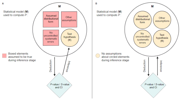
"Emphasizing unconditional interpretations helps avoid overconfident and misleading inferences in light of uncertainties about the assumptions used to arrive at the statistical results." (Greenland et al. 2022).
Note: The term "conditional" as used by Rafi and Greenland probably has a slightly different meaning than normally. "Conditional" in this notion means that all model assumptions are taken as given - it should not be confused with terms like "conditional probability". See also Greenland et al. 2022 for a detailed elaboration on this issue.
In other words, the term compatibility interval emphasizes "the dependence of the p-value on the assumptions as well as on the data, recognizing that p<0.05 can arise from assumption violations even if the effect under study is null" (Gelman/Greenland 2019).
Probabilistic interpretation of p-values and compatibility intervals
Schweder (2018) resp. Schweder and Hjort (2016) (and others) argue that
confidence curves (as produced by p_function()) have a valid probabilistic
interpretation. They distinguish between aleatory probability, which
describes the aleatory stochastic element of a distribution ex ante, i.e.
before the data are obtained. This is the classical interpretation of
confidence intervals following the Neyman-Pearson school of statistics.
However, there is also an ex post probability, called epistemic probability,
for confidence curves. The shift in terminology from confidence intervals
to compatibility intervals may help emphasizing this interpretation.
In this sense, the probabilistic interpretation of p-values and compatibility intervals is "conditional" - on the data and model assumptions (which is in line with the "unconditional" interpretation in the sense of Rafi and Greenland).
Ascribing a probabilistic interpretation to one realized confidence interval is possible without repeated sampling of the specific experiment. Important is the assumption that a sampling distribution is a good description of the variability of the parameter (Vos and Holbert 2022). At the core, the interpretation of a confidence interval is "I assume that this sampling distribution is a good description of the uncertainty of the parameter. If that's a good assumption, then the values in this interval are the most plausible or compatible with the data". The source of confidence in probability statements is the assumption that the selected sampling distribution is appropriate.
"The realized confidence distribution is clearly an epistemic probability distribution" (Schweder 2018). In Bayesian words, compatibility intervals (or confidence distributons, or consonance curves) are "posteriors without priors" (Schweder, Hjort, 2003).
The p-value indicates the degree of compatibility of the endpoints of the
interval at a given confidence level with (1) the observed data and (2) model
assumptions. The observed point estimate (p-value = 1) is the value
estimated to be most compatible with the data and model assumptions,
whereas values values far from the observed point estimate (where p
approaches 0) are least compatible with the data and model assumptions
(Schweder and Hjort 2016, pp. 60-61; Amrhein and Greenland 2022). In this
regards, p-values are statements about confidence or compatibility:
The p-value is not an absolute measure of evidence for a model (such as the
null/alternative model), it is a continuous measure of the compatibility of
the observed data with the model used to compute it (Greenland et al. 2016,
Greenland 2023). Going one step further, and following Schweder, p-values
can be considered as epistemic probability - "not necessarily of the
hypothesis being true, but of it possibly being true" (Schweder 2018).
Hence, the interpretation of p-values might be guided using
bayestestR::p_to_pd().
Probability or compatibility?
We here presented the discussion of p-values and confidence intervals from the perspective of two paradigms, one saying that probability statements can be made, one saying that interpretation is guided in terms of "compatibility". Cox and Hinkley say, "interval estimates cannot be taken as probability statements" (Cox and Hinkley 1979: 208), which conflicts with the Schweder and Hjort confidence distribution school. However, if you view interval estimates as being intervals of values being consistent with the data, this comes close to the idea of (epistemic) probability. We do not believe that these two paradigms contradict or exclude each other. Rather, the aim is to emphasize the one point of view or the other, i.e. to place the linguistic nuances either on 'compatibility' or 'probability'.
The main take-away is not to interpret p-values as dichotomous decisions that distinguish between "we found an effect" (statistically significant)" vs. "we found no effect" (statistically not significant) (Altman and Bland 1995).
Compatibility intervals - is their interpretation "conditional" or not?
The fact that the term "conditional" is used in different meanings in statistics, is confusing. Thus, we would summarize the (probabilistic) interpretation of compatibility intervals as follows: The intervals are built from the data and our modeling assumptions. The accuracy of the intervals depends on our model assumptions. If a value is outside the interval, that might be because (1) that parameter value isn't supported by the data, or (2) the modeling assumptions are a poor fit for the situation. When we make bad assumptions, the compatibility interval might be too wide or (more commonly and seriously) too narrow, making us think we know more about the parameter than is warranted.
When we say "there is a 95% chance the true value is in the interval", that is a statement of epistemic probability (i.e. description of uncertainty related to our knowledge or belief). When we talk about repeated samples or sampling distributions, that is referring to aleatoric (physical properties) probability. Frequentist inference is built on defining estimators with known aleatoric probability properties, from which we can draw epistemic probabilistic statements of uncertainty (Schweder and Hjort 2016).
Functions in the parameters package to check for effect existence and significance
The parameters package provides several options or functions to aid
statistical inference. Beyond p_function(), there are, for example:
-
equivalence_test(), to compute the (conditional) equivalence test for frequentist models -
p_significance(), to compute the probability of practical significance, which can be conceptualized as a unidirectional equivalence test the
pdargument (settingpd = TRUE) inmodel_parameters()includes a column with the probability of direction, i.e. the probability that a parameter is strictly positive or negative. SeebayestestR::p_direction()for details. If plotting is desired, thep_direction()function can be used, together withplot().the
s_valueargument (settings_value = TRUE) inmodel_parameters()replaces the p-values with their related S-values (Rafi and Greenland 2020)finally, it is possible to generate distributions of model coefficients by generating bootstrap-samples (setting
bootstrap = TRUE) or simulating draws from model coefficients usingsimulate_model(). These samples can then be treated as "posterior samples" and used in many functions from the bayestestR package.
Value
A data frame with p-values and compatibility intervals.
Note
Curently, p_function() computes intervals based on Wald t- or z-statistic.
For certain models (like mixed models), profiled intervals may be more
accurate, however, this is currently not supported.
References
Altman DG, Bland JM. Absence of evidence is not evidence of absence. BMJ. 1995;311(7003):485. doi:10.1136/bmj.311.7003.485
Amrhein V, Greenland S. Discuss practical importance of results based on interval estimates and p-value functions, not only on point estimates and null p-values. Journal of Information Technology 2022;37:316–20. doi:10.1177/02683962221105904
Cox DR, Hinkley DV. 1979. Theoretical Statistics. 6th edition. Chapman and Hall/CRC
Fraser DAS. The P-value function and statistical inference. The American Statistician. 2019;73(sup1):135-147. doi:10.1080/00031305.2018.1556735
Gelman A, Greenland S. Are confidence intervals better termed "uncertainty intervals"? BMJ (2019)l5381. doi:10.1136/bmj.l5381
Greenland S, Rafi Z, Matthews R, Higgs M. To Aid Scientific Inference, Emphasize Unconditional Compatibility Descriptions of Statistics. (2022) https://arxiv.org/abs/1909.08583v7 (Accessed November 10, 2022)
Greenland S, Senn SJ, Rothman KJ, Carlin JB, Poole C, Goodman SN, et al. (2016). Statistical tests, P values, confidence intervals, and power: A guide to misinterpretations. European Journal of Epidemiology. 31:337-350. doi:10.1007/s10654-016-0149-3
Greenland S (2023). Divergence versus decision P-values: A distinction worth making in theory and keeping in practice: Or, how divergence P-values measure evidence even when decision P-values do not. Scand J Statist, 50(1), 54-88.
Rafi Z, Greenland S. Semantic and cognitive tools to aid statistical science: Replace confidence and significance by compatibility and surprise. BMC Medical Research Methodology. 2020;20(1):244. doi:10.1186/s12874-020-01105-9
Schweder T. Confidence is epistemic probability for empirical science. Journal of Statistical Planning and Inference (2018) 195:116–125. doi:10.1016/j.jspi.2017.09.016
Schweder T, Hjort NL. Confidence and Likelihood. Scandinavian Journal of Statistics. 2002;29(2):309-332. doi:10.1111/1467-9469.00285
Schweder T, Hjort NL. Frequentist analogues of priors and posteriors. In Stigum, B. (ed.), Econometrics and the Philosophy of Economics: Theory Data Confrontation in Economics, pp. 285-217. Princeton University Press, Princeton, NJ, 2003
Schweder T, Hjort NL. Confidence, Likelihood, Probability: Statistical inference with confidence distributions. Cambridge University Press, 2016.
Vos P, Holbert D. Frequentist statistical inference without repeated sampling. Synthese 200, 89 (2022). doi:10.1007/s11229-022-03560-x
See Also
See also equivalence_test() and p_significance() for
functions related to checking effect existence and significance.
Examples
model <- lm(Sepal.Length ~ Species, data = iris)
p_function(model)

model <- lm(mpg ~ wt + as.factor(gear) + am, data = mtcars)
result <- p_function(model)

# single panels
plot(result, n_columns = 2)

# integrated plot, the default
plot(result)
Practical Significance (ps)
Description
Compute the probability of Practical Significance (ps), which can be conceptualized as a unidirectional equivalence test. It returns the probability that an effect is above a given threshold corresponding to a negligible effect in the median's direction, considering a parameter's full confidence interval. In other words, it returns the probability of a clear direction of an effect, which is larger than the smallest effect size of interest (e.g., a minimal important difference). Its theoretical range is from zero to one, but the ps is typically larger than 0.5 (to indicate practical significance).
In comparison the the equivalence_test() function, where the SGPV
(second generation p-value) describes the proportion of the full confidence
interval that is inside the ROPE, the value returned by p_significance()
describes the larger proportion of the full confidence interval that is
outside the ROPE. This makes p_significance() comparable to
bayestestR::p_direction(), however, while p_direction() compares to a
point-null by default, p_significance() compares to a range-null.
Usage
## S3 method for class 'lm'
p_significance(
  x,
  threshold = "default",
  ci = 0.95,
  vcov = NULL,
  vcov_args = NULL,
  verbose = TRUE,
  ...
)
Arguments
x |
A statistical model. |
threshold |
The threshold value that separates significant from negligible effect, which can have following possible values:
|
ci |
Confidence Interval (CI) level. Default to |
vcov |
Variance-covariance matrix used to compute uncertainty estimates (e.g., for robust standard errors). This argument accepts a covariance matrix, a function which returns a covariance matrix, or a string which identifies the function to be used to compute the covariance matrix.
|
vcov_args |
List of arguments to be passed to the function identified by
the |
verbose |
Toggle warnings and messages. |
... |
Arguments passed to other methods. |
Details
p_significance() returns the proportion of the full confidence
interval range (assuming a normally or t-distributed, equal-tailed interval,
based on the model) that is outside a certain range (the negligible effect,
or ROPE, see argument threshold). If there are values of the distribution
both below and above the ROPE, p_significance() returns the higher
probability of a value being outside the ROPE. Typically, this value should
be larger than 0.5 to indicate practical significance. However, if the range
of the negligible effect is rather large compared to the range of the
confidence interval, p_significance() will be less than 0.5, which
indicates no clear practical significance.
Note that the assumed interval, which is used to calculate the practical significance, is an estimation of the full interval based on the chosen confidence level. For example, if the 95% confidence interval of a coefficient ranges from -1 to 1, the underlying full (normally or t-distributed) interval approximately ranges from -1.9 to 1.9, see also following code:
# simulate full normal distribution
out <- bayestestR::distribution_normal(10000, 0, 0.5)
# range of "full" distribution
range(out)
# range of 95% CI
round(quantile(out, probs = c(0.025, 0.975)), 2)
This ensures that the practical significance always refers to the general compatible parameter space of coefficients. Therefore, the full interval is similar to a Bayesian posterior distribution of an equivalent Bayesian model, see following code:
library(bayestestR)
library(brms)
m <- lm(mpg ~ gear + wt + cyl + hp, data = mtcars)
m2 <- brm(mpg ~ gear + wt + cyl + hp, data = mtcars)
# probability of significance (ps) for frequentist model
p_significance(m)
# similar to ps of Bayesian models
p_significance(m2)
# similar to ps of simulated draws / bootstrap samples
p_significance(simulate_model(m))
Value
A data frame with columns for the parameter names, the confidence intervals and the values for practical significance. Higher values indicate more practical significance (upper bound is one).
Statistical inference - how to quantify evidence
There is no standardized approach to drawing conclusions based on the available data and statistical models. A frequently chosen but also much criticized approach is to evaluate results based on their statistical significance (Amrhein et al. 2017).
A more sophisticated way would be to test whether estimated effects exceed the "smallest effect size of interest", to avoid even the smallest effects being considered relevant simply because they are statistically significant, but clinically or practically irrelevant (Lakens et al. 2018, Lakens 2024).
A rather unconventional approach, which is nevertheless advocated by various authors, is to interpret results from classical regression models either in terms of probabilities, similar to the usual approach in Bayesian statistics (Schweder 2018; Schweder and Hjort 2003; Vos 2022) or in terms of relative measure of "evidence" or "compatibility" with the data (Greenland et al. 2022; Rafi and Greenland 2020), which nevertheless comes close to a probabilistic interpretation.
A more detailed discussion of this topic is found in the documentation of
p_function().
The parameters package provides several options or functions to aid statistical inference. These are, for example:
-
equivalence_test(), to compute the (conditional) equivalence test for frequentist models -
p_significance(), to compute the probability of practical significance, which can be conceptualized as a unidirectional equivalence test -
p_function(), or consonance function, to compute p-values and compatibility (confidence) intervals for statistical models the
pdargument (settingpd = TRUE) inmodel_parameters()includes a column with the probability of direction, i.e. the probability that a parameter is strictly positive or negative. SeebayestestR::p_direction()for details. If plotting is desired, thep_direction()function can be used, together withplot().the
s_valueargument (settings_value = TRUE) inmodel_parameters()replaces the p-values with their related S-values (Rafi and Greenland 2020)finally, it is possible to generate distributions of model coefficients by generating bootstrap-samples (setting
bootstrap = TRUE) or simulating draws from model coefficients usingsimulate_model(). These samples can then be treated as "posterior samples" and used in many functions from the bayestestR package.
Most of the above shown options or functions derive from methods originally
implemented for Bayesian models (Makowski et al. 2019). However, assuming
that model assumptions are met (which means, the model fits well to the data,
the correct model is chosen that reflects the data generating process
(distributional model family) etc.), it seems appropriate to interpret
results from classical frequentist models in a "Bayesian way" (more details:
documentation in p_function()).
Note
There is also a plot()-method
implemented in the see-package.
References
Amrhein, V., Korner-Nievergelt, F., and Roth, T. (2017). The earth is flat (p > 0.05): Significance thresholds and the crisis of unreplicable research. PeerJ, 5, e3544. doi:10.7717/peerj.3544
Greenland S, Rafi Z, Matthews R, Higgs M. To Aid Scientific Inference, Emphasize Unconditional Compatibility Descriptions of Statistics. (2022) https://arxiv.org/abs/1909.08583v7 (Accessed November 10, 2022)
Lakens, D. (2024). Improving Your Statistical Inferences (Version v1.5.1). Retrieved from https://lakens.github.io/statistical_inferences/. doi:10.5281/ZENODO.6409077
Lakens, D., Scheel, A. M., and Isager, P. M. (2018). Equivalence Testing for Psychological Research: A Tutorial. Advances in Methods and Practices in Psychological Science, 1(2), 259–269.
Makowski, D., Ben-Shachar, M. S., Chen, S. H. A., and Lüdecke, D. (2019). Indices of Effect Existence and Significance in the Bayesian Framework. Frontiers in Psychology, 10, 2767. doi:10.3389/fpsyg.2019.02767
Rafi Z, Greenland S. Semantic and cognitive tools to aid statistical science: replace confidence and significance by compatibility and surprise. BMC Medical Research Methodology (2020) 20:244.
Schweder T. Confidence is epistemic probability for empirical science. Journal of Statistical Planning and Inference (2018) 195:116–125. doi:10.1016/j.jspi.2017.09.016
Schweder T, Hjort NL. Frequentist analogues of priors and posteriors. In Stigum, B. (ed.), Econometrics and the Philosophy of Economics: Theory Data Confrontation in Economics, pp. 285-217. Princeton University Press, Princeton, NJ, 2003
Vos P, Holbert D. Frequentist statistical inference without repeated sampling. Synthese 200, 89 (2022). doi:10.1007/s11229-022-03560-x
See Also
For more details, see bayestestR::p_significance(). See also
equivalence_test(), p_function() and bayestestR::p_direction()
for functions related to checking effect existence and significance.
Examples
data(qol_cancer)
model <- lm(QoL ~ time + age + education, data = qol_cancer)

p_significance(model)
p_significance(model, threshold = c(-0.5, 1.5))

# based on heteroscedasticity-robust standard errors
p_significance(model, vcov = "HC3")

if (require("see", quietly = TRUE)) {
  result <- p_significance(model)
  plot(result)
}
p-values
Description
This function attempts to return, or compute, p-values of a model's parameters.
Usage
p_value(model, ...)

## Default S3 method:
p_value(
  model,
  dof = NULL,
  method = NULL,
  component = "all",
  vcov = NULL,
  vcov_args = NULL,
  verbose = TRUE,
  ...
)

## S3 method for class 'emmGrid'
p_value(model, ci = 0.95, adjust = "none", ...)

## S3 method for class 'gam'
p_value(model, re_test = TRUE, ...)
Arguments
model |
A statistical model. |
... |
Additional arguments |
dof |
Number of degrees of freedom to be used when calculating
confidence intervals. If |
method |
Method for computing degrees of freedom for confidence
intervals (CI) and the related p-values. Allowed are following options (which
vary depending on the model class): |
component |
Model component for which parameters should be shown. See
the documentation for your object's class in |
vcov |
Variance-covariance matrix used to compute uncertainty estimates (e.g., for robust standard errors). This argument accepts a covariance matrix, a function which returns a covariance matrix, or a string which identifies the function to be used to compute the covariance matrix.
|
vcov_args |
List of arguments to be passed to the function identified by
the |
verbose |
Toggle warnings and messages. |
ci |
Confidence Interval (CI) level. Default to |
adjust |
Character value naming the method used to adjust p-values or
confidence intervals. See |
re_test |
Logical, if |
Details
For Bayesian models, the p-values corresponds to the probability of
direction (bayestestR::p_direction()), which is converted to a p-value
using bayestestR::convert_pd_to_p().
Value
A data frame with at least two columns: the parameter names and the p-values. Depending on the model, may also include columns for model components etc.
Confidence intervals and approximation of degrees of freedom
There are different ways of approximating the degrees of freedom depending
on different assumptions about the nature of the model and its sampling
distribution. The ci_method argument modulates the method for computing degrees
of freedom (df) that are used to calculate confidence intervals (CI) and the
related p-values. Following options are allowed, depending on the model
class:
Classical methods:
Classical inference is generally based on the Wald method. The Wald approach to inference computes a test statistic by dividing the parameter estimate by its standard error (Coefficient / SE), then comparing this statistic against a t- or normal distribution. This approach can be used to compute CIs and p-values.
"wald":
Applies to non-Bayesian models. For linear models, CIs computed using the Wald method (SE and a t-distribution with residual df); p-values computed using the Wald method with a t-distribution with residual df. For other models, CIs computed using the Wald method (SE and a normal distribution); p-values computed using the Wald method with a normal distribution.
"normal"
Applies to non-Bayesian models. Compute Wald CIs and p-values, but always use a normal distribution.
"residual"
Applies to non-Bayesian models. Compute Wald CIs and p-values, but always use a t-distribution with residual df when possible. If the residual df for a model cannot be determined, a normal distribution is used instead.
Methods for mixed models:
Compared to fixed effects (or single-level) models, determining appropriate df for Wald-based inference in mixed models is more difficult. See the R GLMM FAQ for a discussion.
Several approximate methods for computing df are available, but you should
also consider instead using profile likelihood ("profile") or bootstrap ("boot")
CIs and p-values instead.
"satterthwaite"
Applies to linear mixed models. CIs computed using the Wald method (SE and a t-distribution with Satterthwaite df); p-values computed using the Wald method with a t-distribution with Satterthwaite df.
"kenward"
Applies to linear mixed models. CIs computed using the Wald method (Kenward-Roger SE and a t-distribution with Kenward-Roger df); p-values computed using the Wald method with Kenward-Roger SE and t-distribution with Kenward-Roger df.
"ml1"
Applies to linear mixed models. CIs computed using the Wald method (SE and a t-distribution with m-l-1 approximated df); p-values computed using the Wald method with a t-distribution with m-l-1 approximated df. See
ci_ml1().
"betwithin"
Applies to linear mixed models and generalized linear mixed models. CIs computed using the Wald method (SE and a t-distribution with between-within df); p-values computed using the Wald method with a t-distribution with between-within df. See
ci_betwithin().
Likelihood-based methods:
Likelihood-based inference is based on comparing the likelihood for the
maximum-likelihood estimate to the the likelihood for models with one or more
parameter values changed (e.g., set to zero or a range of alternative values).
Likelihood ratios for the maximum-likelihood and alternative models are compared
to a \chi-squared distribution to compute CIs and p-values.
"profile"
Applies to non-Bayesian models of class
glm,polr,merModorglmmTMB. CIs computed by profiling the likelihood curve for a parameter, using linear interpolation to find where likelihood ratio equals a critical value; p-values computed using the Wald method with a normal-distribution (note: this might change in a future update!)
"uniroot"
Applies to non-Bayesian models of class
glmmTMB. CIs computed by profiling the likelihood curve for a parameter, using root finding to find where likelihood ratio equals a critical value; p-values computed using the Wald method with a normal-distribution (note: this might change in a future update!)
Methods for bootstrapped or Bayesian models:
Bootstrap-based inference is based on resampling and refitting the model to the resampled datasets. The distribution of parameter estimates across resampled datasets is used to approximate the parameter's sampling distribution. Depending on the type of model, several different methods for bootstrapping and constructing CIs and p-values from the bootstrap distribution are available.
For Bayesian models, inference is based on drawing samples from the model posterior distribution.
"quantile" (or "eti")
Applies to all models (including Bayesian models). For non-Bayesian models, only applies if
bootstrap = TRUE. CIs computed as equal tailed intervals using the quantiles of the bootstrap or posterior samples; p-values are based on the probability of direction. SeebayestestR::eti().
"hdi"
Applies to all models (including Bayesian models). For non-Bayesian models, only applies if
bootstrap = TRUE. CIs computed as highest density intervals for the bootstrap or posterior samples; p-values are based on the probability of direction. SeebayestestR::hdi().
"bci" (or "bcai")
Applies to all models (including Bayesian models). For non-Bayesian models, only applies if
bootstrap = TRUE. CIs computed as bias corrected and accelerated intervals for the bootstrap or posterior samples; p-values are based on the probability of direction. SeebayestestR::bci().
"si"
Applies to Bayesian models with proper priors. CIs computed as support intervals comparing the posterior samples against the prior samples; p-values are based on the probability of direction. See
bayestestR::si().
"boot"
Applies to non-Bayesian models of class
merMod. CIs computed using parametric bootstrapping (simulating data from the fitted model); p-values computed using the Wald method with a normal-distribution) (note: this might change in a future update!).
For all iteration-based methods other than "boot"
("hdi", "quantile", "ci", "eti", "si", "bci", "bcai"),
p-values are based on the probability of direction (bayestestR::p_direction()),
which is converted into a p-value using bayestestR::pd_to_p().
Model components
Possible values for the component argument depend on the model class.
Following are valid options:
-
"all": returns all model components, applies to all models, but will only have an effect for models with more than just the conditional model component. -
"conditional": only returns the conditional component, i.e. "fixed effects" terms from the model. Will only have an effect for models with more than just the conditional model component. -
"smooth_terms": returns smooth terms, only applies to GAMs (or similar models that may contain smooth terms). -
"zero_inflated"(or"zi"): returns the zero-inflation component. -
"dispersion": returns the dispersion model component. This is common for models with zero-inflation or that can model the dispersion parameter. -
"instruments": for instrumental-variable or some fixed effects regression, returns the instruments. -
"nonlinear": for non-linear models (like models of classnlmerModornls), returns staring estimates for the nonlinear parameters. -
"correlation": for models with correlation-component, likegls, the variables used to describe the correlation structure are returned.
Special models
Some model classes also allow rather uncommon options. These are:
-
mhurdle:
"infrequent_purchase","ip", and"auxiliary" -
BGGM:
"correlation"and"intercept" -
BFBayesFactor, glmx:
"extra" -
averaging:
"conditional"and"full" -
mjoint:
"survival" -
mfx:
"precision","marginal" -
betareg, DirichletRegModel:
"precision" -
mvord:
"thresholds"and"correlation" -
clm2:
"scale" -
selection:
"selection","outcome", and"auxiliary" -
lavaan: One or more of
"regression","correlation","loading","variance","defined", or"mean". Can also be"all"to include all components.
For models of class brmsfit (package brms), even more options are
possible for the component argument, which are not all documented in detail
here.
Examples
data(iris)
model <- lm(Petal.Length ~ Sepal.Length + Species, data = iris)
p_value(model)

data("bioChemists", package = "pscl")
model <- pscl::zeroinfl(
  art ~ fem + mar + kid5 | kid5 + phd,
  data = bioChemists
)
p_value(model)
p_value(model, component = "zi")
Global options from the parameters package
Description
Global options from the parameters package
Global options to set defaults for function arguments
The verbose argument can be used to display or silence messages and
warnings for the different functions in the parameters package. However,
some messages providing additional information can be displayed or suppressed
using options():
-
options(parameters_info = TRUE)will override theinclude_infoargument inmodel_parameters()and always show the model summary for non-mixed models. -
options(parameters_mixed_info = TRUE)will override theinclude_infoargument inmodel_parameters()for mixed models, and will then always show the model summary. -
options(parameters_cimethod = TRUE)will show the additional information about the approximation method used to calculate confidence intervals and p-values. Set toFALSEto hide this message when printingmodel_parameters()objects. -
options(parameters_exponentiate = TRUE)will show the additional information on how to interpret coefficients of models with log-transformed response variables or with log-/logit-links when theexponentiateargument inmodel_parameters()is notTRUE. Set this option toFALSEto hide this message when printingmodel_parameters()objects.
There are further options that can be used to modify the default behaviour for printed outputs:
-
options(parameters_labels = TRUE)will use variable and value labels for pretty names, if data is labelled. If no labels available, default pretty names are used. -
options(parameters_interaction = <character>)will replace the interaction mark (by default,*) with the related character. -
options(parameters_select = <value>)will set the default for theselectargument. See argument's documentation for available options. -
options(easystats_table_width = <value>)will set the default width for tables in text-format, i.e. for most of the outputs printed to console. If not specified, tables will be adjusted to the current available width, e.g. of the of the console (or any other source for textual output, like markdown files). The argumenttable_widthcan also be used in mostprint()methods to specify the table width as desired. -
options(insight_use_symbols = TRUE)will try to print unicode-chars for symbols as column names, wherever possible (e.g., ω instead ofOmega). -
options(easystats_display_format = <value>)will set the default format for thedisplay()methods. Can be one of"markdown","html", or"tt". Seedisplay.parameters_model()for details.
Type of model parameters
Description
In a regression model, the parameters do not all have the meaning. For
instance, the intercept has to be interpreted as theoretical outcome value
under some conditions (when predictors are set to 0), whereas other
coefficients are to be interpreted as amounts of change. Others, such as
interactions, represent changes in another of the parameter. The
parameters_type function attempts to retrieve information and meaning
of parameters. It outputs a dataframe of information for each parameters,
such as the Type (whether the parameter corresponds to a factor or a
numeric predictor, or whether it is a (regular) interaction or a nested
one), the Link (whether the parameter can be interpreted as a mean
value, the slope of an association or a difference between two levels) and,
in the case of interactions, which other parameters is impacted by which
parameter.
Usage
parameters_type(model, ...)
Arguments
model |
A statistical model. |
... |
Arguments passed to or from other methods. |
Value
A data frame.
Examples
library(parameters)

model <- lm(Sepal.Length ~ Petal.Length + Species, data = iris)
parameters_type(model)

model <- lm(Sepal.Length ~ Species + poly(Sepal.Width, 2), data = iris)
parameters_type(model)

model <- lm(Sepal.Length ~ Species + poly(Sepal.Width, 2, raw = TRUE), data = iris)
parameters_type(model)

# Interactions
model <- lm(Sepal.Length ~ Sepal.Width * Species, data = iris)
parameters_type(model)

model <- lm(Sepal.Length ~ Sepal.Width * Species * Petal.Length, data = iris)
parameters_type(model)

model <- lm(Sepal.Length ~ Species * Sepal.Width, data = iris)
parameters_type(model)

model <- lm(Sepal.Length ~ Species / Sepal.Width, data = iris)
parameters_type(model)


# Complex interactions
data <- iris
data$fac2 <- ifelse(data$Sepal.Width > mean(data$Sepal.Width), "A", "B")
model <- lm(Sepal.Length ~ Species / fac2 / Petal.Length, data = data)
parameters_type(model)

model <- lm(Sepal.Length ~ Species / fac2 * Petal.Length, data = data)
parameters_type(model)
Pool Model Parameters
Description
This function "pools" (i.e. combines) model parameters in a similar fashion
as mice::pool(). However, this function pools parameters from
parameters_model objects, as returned by
model_parameters().
Usage
pool_parameters(
  x,
  exponentiate = FALSE,
  effects = "fixed",
  component = "all",
  verbose = TRUE,
  ...
)
Arguments
x |
A list of |
exponentiate |
Logical, indicating whether or not to exponentiate the
coefficients (and related confidence intervals). This is typical for
logistic regression, or more generally speaking, for models with log or
logit links. It is also recommended to use |
effects |
Should parameters for fixed effects ( |
component |
Which type of parameters to return, such as parameters for the
conditional model, the zero-inflation part of the model, the dispersion
term, or other auxiliary parameters be returned? Applies to models with
zero-inflation and/or dispersion formula, or if parameters such as |
verbose |
Toggle warnings and messages. |
... |
Arguments passed down to |
Details
Averaging of parameters follows Rubin's rules (Rubin, 1987, p. 76). The pooled degrees of freedom is based on the Barnard-Rubin adjustment for small samples (Barnard and Rubin, 1999).
Value
A data frame of indices related to the model's parameters.
Note
Models with multiple components, (for instance, models with zero-inflation,
where predictors appear in the count and zero-inflation part, or models with
dispersion component) may fail in rare situations. In this case, compute
the pooled parameters for components separately, using the component
argument.
Some model objects do not return standard errors (e.g. objects of class
htest). For these models, no pooled confidence intervals nor p-values
are returned.
References
Barnard, J. and Rubin, D.B. (1999). Small sample degrees of freedom with multiple imputation. Biometrika, 86, 948-955. Rubin, D.B. (1987). Multiple Imputation for Nonresponse in Surveys. New York: John Wiley and Sons.
Examples
# example for multiple imputed datasets
data("nhanes2", package = "mice")
imp <- mice::mice(nhanes2, printFlag = FALSE)
models <- lapply(1:5, function(i) {
  lm(bmi ~ age + hyp + chl, data = mice::complete(imp, action = i))
})
pool_parameters(models)

# should be identical to:
m <- with(data = imp, exp = lm(bmi ~ age + hyp + chl))
summary(mice::pool(m))

# For glm, mice used residual df, while `pool_parameters()` uses `Inf`
nhanes2$hyp <- datawizard::slide(as.numeric(nhanes2$hyp))
imp <- mice::mice(nhanes2, printFlag = FALSE)
models <- lapply(1:5, function(i) {
  glm(hyp ~ age + chl, family = binomial, data = mice::complete(imp, action = i))
})
m <- with(data = imp, exp = glm(hyp ~ age + chl, family = binomial))
# residual df
summary(mice::pool(m))$df
# df = Inf
pool_parameters(models)$df_error
# use residual df instead
pool_parameters(models, ci_method = "residual")$df_error
Predict method for parameters_clusters objects
Description
Predict method for parameters_clusters objects
Usage
## S3 method for class 'parameters_clusters'
predict(object, newdata = NULL, names = NULL, ...)
Arguments
object |
a model object for which prediction is desired. |
newdata |
data.frame |
names |
character vector or list |
... |
additional arguments affecting the predictions produced. |
Sample data set
Description
A sample data set with longitudinal data, used in the vignette describing the datawizard::demean() function. Health-related quality of life from cancer-patients was measured at three time points (pre-surgery, 6 and 12 months after surgery).
Format
A data frame with 564 rows and 7 variables:
- ID
Patient ID
- QoL
Quality of Life Score
- time
Timepoint of measurement
- age
Age in years
- phq4
Patients' Health Questionnaire, 4-item version
- hospital
Hospital ID, where patient was treated
- education
Patients' educational level
Summary information from random effects
Description
This function extracts the different variance components of a mixed model and returns the result as a data frame.
Usage
random_parameters(model, component = "conditional")
Arguments
model |
A mixed effects model (including |
component |
Should all parameters, parameters for the conditional model,
for the zero-inflation part of the model, or the dispersion model be returned?
Applies to models with zero-inflation and/or dispersion component. |
Details
The variance components are obtained from insight::get_variance() and
are denoted as following:
Within-group (or residual) variance
The residual variance, σ2ε, is the sum of the distribution-specific variance and the variance due to additive dispersion. It indicates the within-group variance.
Between-group random intercept variance
The random intercept variance, or between-group variance
for the intercept (τ00),
is obtained from VarCorr(). It indicates how much groups
or subjects differ from each other.
Between-group random slope variance
The random slope variance, or between-group variance
for the slopes (τ11)
is obtained from VarCorr(). This measure is only available
for mixed models with random slopes. It indicates how much groups
or subjects differ from each other according to their slopes.
Random slope-intercept correlation
The random slope-intercept correlation
(ρ01)
is obtained from VarCorr(). This measure is only available
for mixed models with random intercepts and slopes.
Note: For the within-group and between-group variance, variance and standard deviations (which are simply the square root of the variance) are shown.
Value
A data frame with random effects statistics for the variance components, including number of levels per random effect group, as well as complete observations in the model.
Examples
if (require("lme4")) {
  data(sleepstudy)
  model <- lmer(Reaction ~ Days + (1 + Days | Subject), data = sleepstudy)
  random_parameters(model)
}
Dimensionality reduction (DR) / Features Reduction
Description
This function performs a reduction in the parameter space (the number of
variables). It starts by creating a new set of variables, based on the given
method (the default method is "PCA", but other are available via the
method argument, such as "cMDS", "DRR" or "ICA"). Then, it names this
new dimensions using the original variables that correlates the most with it.
For instance, a variable named 'V1_0.97/V4_-0.88' means that the V1 and the
V4 variables correlate maximally (with respective coefficients of .97 and
-.88) with this dimension. Although this function can be useful in
exploratory data analysis, it's best to perform the dimension reduction step
in a separate and dedicated stage, as this is a very important process in the
data analysis workflow. reduce_data() is an alias for
reduce_parameters.data.frame().
Usage
reduce_parameters(x, method = "PCA", n = "max", distance = "euclidean", ...)

reduce_data(x, method = "PCA", n = "max", distance = "euclidean", ...)
Arguments
x |
A data frame or a statistical model. For |
method |
The feature reduction method. Can be one of |
n |
Number of components to extract. If |
distance |
The distance measure to be used. Only applies when
|
... |
Arguments passed to or from other methods. |
Details
The different methods available are described below:
Supervised Methods
-
PCA: See
principal_components(). -
cMDS / PCoA: Classical Multidimensional Scaling (cMDS) takes a set of dissimilarities (i.e., a distance matrix) and returns a set of points such that the distances between the points are approximately equal to the dissimilarities.
-
DRR: Dimensionality Reduction via Regression (DRR) is a very recent technique extending PCA (Laparra et al., 2015). Starting from a rotated PCA, it predicts redundant information from the remaining components using non-linear regression. Some of the most notable advantages of performing DRR are avoidance of multicollinearity between predictors and overfitting mitigation. DRR tends to perform well when the first principal component is enough to explain most of the variation in the predictors. Requires the DRR package to be installed.
-
ICA: Performs an Independent Component Analysis using the FastICA algorithm. Contrary to PCA, which attempts to find uncorrelated sources (through least squares minimization), ICA attempts to find independent sources, i.e., the source space that maximizes the "non-gaussianity" of all sources. Contrary to PCA, ICA does not rank each source, which makes it a poor tool for dimensionality reduction. Requires the fastICA package to be installed.
See also package vignette.
References
Nguyen, L. H., and Holmes, S. (2019). Ten quick tips for effective dimensionality reduction. PLOS Computational Biology, 15(6).
Laparra, V., Malo, J., and Camps-Valls, G. (2015). Dimensionality reduction via regression in hyperspectral imagery. IEEE Journal of Selected Topics in Signal Processing, 9(6), 1026-1036.
Examples
data(iris)
model <- lm(Sepal.Width ~ Species * Sepal.Length + Petal.Width, data = iris)
model
reduce_parameters(model)

out <- reduce_data(iris, method = "PCA", n = "max")
head(out)
Objects exported from other packages
Description
These objects are imported from other packages. Follow the links below to see their documentation.
- bayestestR
- datawizard
demean(),describe_distribution(),kurtosis(),rescale_weights(),skewness(),visualisation_recipe()- insight
display(),n_parameters(),print_html(),print_md(),standardize_names(),supported_models()
Reshape loadings between wide/long formats
Description
Reshape loadings between wide/long formats.
Usage
reshape_loadings(x, ...)

## S3 method for class 'parameters_efa'
reshape_loadings(x, threshold = NULL, ...)

## S3 method for class 'data.frame'
reshape_loadings(x, threshold = NULL, loadings_columns = NULL, ...)
Arguments
x |
A data frame or a statistical model. For |
... |
Arguments passed to or from other methods. |
threshold |
A value between 0 and 1 indicates which (absolute) values
from the loadings should be removed. An integer higher than 1 indicates the
n strongest loadings to retain. Can also be |
loadings_columns |
Vector indicating the columns corresponding to loadings. |
Examples
if (require("psych")) {
  pca <- model_parameters(psych::fa(attitude, nfactors = 3))
  loadings <- reshape_loadings(pca)

  loadings
  reshape_loadings(loadings)
}
Automated selection of model parameters
Description
This function performs an automated selection of the 'best' parameters, updating and returning the "best" model.
Usage
select_parameters(model, ...)

## S3 method for class 'lm'
select_parameters(model, direction = "both", steps = 1000, k = 2, ...)

## S3 method for class 'merMod'
select_parameters(model, direction = "backward", steps = 1000, ...)
Arguments
model |
A statistical model (of class |
... |
Arguments passed to or from other methods. |
direction |
the mode of stepwise search, can be one of |
steps |
the maximum number of steps to be considered. The default is 1000 (essentially as many as required). It is typically used to stop the process early. |
k |
The multiple of the number of degrees of freedom used for the penalty.
Only |
Value
The model refitted with optimal number of parameters.
Classical lm and glm
For frequentist GLMs, select_parameters() performs an AIC-based stepwise
selection.
Mixed models
For mixed-effects models of class merMod, stepwise selection is based on
cAIC4::stepcAIC(). This step function only searches the "best" model
based on the random-effects structure, i.e. select_parameters() adds or
excludes random-effects until the cAIC can't be improved further.
Examples
model <- lm(mpg ~ ., data = mtcars)
select_parameters(model)

model <- lm(mpg ~ cyl * disp * hp * wt, data = mtcars)
select_parameters(model)

# lme4 -------------------------------------------
model <- lme4::lmer(
  Sepal.Width ~ Sepal.Length * Petal.Width * Petal.Length + (1 | Species),
  data = iris
)
select_parameters(model)
Simulated draws from model coefficients
Description
Simulate draws from a statistical model to return a data frame of estimates.
Usage
simulate_model(model, iterations = 1000, ...)

## Default S3 method:
simulate_model(model, iterations = 1000, component = "all", ...)
Arguments
model |
Statistical model (no Bayesian models). |
iterations |
The number of draws to simulate/bootstrap. |
... |
Arguments passed to |
component |
Should all parameters, parameters for the conditional model,
for the zero-inflation part of the model, or the dispersion model be returned?
Applies to models with zero-inflation and/or dispersion component. |
Details
Technical Details
simulate_model() is a computationally faster alternative
to bootstrap_model(). Simulated draws for coefficients are based
on a multivariate normal distribution (MASS::mvrnorm()) with mean
mu = coef(model) and variance Sigma = vcov(model).
Models with Zero-Inflation Component
For models from packages glmmTMB, pscl, GLMMadaptive and
countreg, the component argument can be used to specify
which parameters should be simulated. For all other models, parameters
from the conditional component (fixed effects) are simulated. This may
include smooth terms, but not random effects.
Value
A data frame.
Model components
Possible values for the component argument depend on the model class.
Following are valid options:
-
"all": returns all model components, applies to all models, but will only have an effect for models with more than just the conditional model component. -
"conditional": only returns the conditional component, i.e. "fixed effects" terms from the model. Will only have an effect for models with more than just the conditional model component. -
"smooth_terms": returns smooth terms, only applies to GAMs (or similar models that may contain smooth terms). -
"zero_inflated"(or"zi"): returns the zero-inflation component. -
"dispersion": returns the dispersion model component. This is common for models with zero-inflation or that can model the dispersion parameter. -
"instruments": for instrumental-variable or some fixed effects regression, returns the instruments. -
"nonlinear": for non-linear models (like models of classnlmerModornls), returns staring estimates for the nonlinear parameters. -
"correlation": for models with correlation-component, likegls, the variables used to describe the correlation structure are returned.
Special models
Some model classes also allow rather uncommon options. These are:
-
mhurdle:
"infrequent_purchase","ip", and"auxiliary" -
BGGM:
"correlation"and"intercept" -
BFBayesFactor, glmx:
"extra" -
averaging:
"conditional"and"full" -
mjoint:
"survival" -
mfx:
"precision","marginal" -
betareg, DirichletRegModel:
"precision" -
mvord:
"thresholds"and"correlation" -
clm2:
"scale" -
selection:
"selection","outcome", and"auxiliary" -
lavaan: One or more of
"regression","correlation","loading","variance","defined", or"mean". Can also be"all"to include all components.
For models of class brmsfit (package brms), even more options are
possible for the component argument, which are not all documented in detail
here.
See Also
simulate_parameters(), bootstrap_model(), bootstrap_parameters()
Examples
model <- lm(Sepal.Length ~ Species * Petal.Width + Petal.Length, data = iris)
head(simulate_model(model))

if (require("glmmTMB", quietly = TRUE)) {
  model <- glmmTMB(
    count ~ spp + mined + (1 | site),
    ziformula = ~mined,
    family = poisson(),
    data = Salamanders
  )
  head(simulate_model(model))
  head(simulate_model(model, component = "zero_inflated"))
}
Simulate Model Parameters
Description
Compute simulated draws of parameters and their related indices such as Confidence Intervals (CI) and p-values. Simulating parameter draws can be seen as a (computationally faster) alternative to bootstrapping.
Usage
simulate_parameters(model, ...)

## Default S3 method:
simulate_parameters(
  model,
  iterations = 1000,
  centrality = "median",
  ci = 0.95,
  ci_method = "quantile",
  test = "p-value",
  ...
)
Arguments
model |
Statistical model (no Bayesian models). |
... |
Arguments passed to |
iterations |
The number of draws to simulate/bootstrap. |
centrality |
The point-estimates (centrality indices) to compute. Character
(vector) or list with one or more of these options: |
ci |
Value or vector of probability of the CI (between 0 and 1)
to be estimated. Default to |
ci_method |
The type of index used for Credible Interval. Can be |
test |
The indices of effect existence to compute. Character (vector) or
list with one or more of these options: |
Details
Technical Details
simulate_parameters() is a computationally faster alternative
to bootstrap_parameters(). Simulated draws for coefficients are based
on a multivariate normal distribution (MASS::mvrnorm()) with mean
mu = coef(model) and variance Sigma = vcov(model).
Models with Zero-Inflation Component
For models from packages glmmTMB, pscl, GLMMadaptive and
countreg, the component argument can be used to specify
which parameters should be simulated. For all other models, parameters
from the conditional component (fixed effects) are simulated. This may
include smooth terms, but not random effects.
Value
A data frame with simulated parameters.
Note
There is also a plot()-method implemented in the see-package.
References
Gelman A, Hill J. Data analysis using regression and multilevel/hierarchical models. Cambridge; New York: Cambridge University Press 2007: 140-143
See Also
bootstrap_model(), bootstrap_parameters(), simulate_model()
Examples
model <- lm(Sepal.Length ~ Species * Petal.Width + Petal.Length, data = iris)
simulate_parameters(model)


if (require("glmmTMB", quietly = TRUE)) {
  model <- glmmTMB(
    count ~ spp + mined + (1 | site),
    ziformula = ~mined,
    family = poisson(),
    data = Salamanders
  )
  simulate_parameters(model, centrality = "mean")
  simulate_parameters(model, ci = c(.8, .95), component = "zero_inflated")
}
Sort parameters by coefficient values
Description
Sort parameters by coefficient values
Usage
sort_parameters(x, ...)

## Default S3 method:
sort_parameters(x, sort = "none", column = "Coefficient", ...)
Arguments
x |
A data frame or a |
... |
Arguments passed to or from other methods. |
sort |
If |
column |
The column containing model parameter estimates. This will be
|
Value
A sorted data frame or original object.
Examples
# creating object to sort (can also be a regular data frame)
mod <- model_parameters(stats::lm(wt ~ am * cyl, data = mtcars))

# original output
mod

# sorted outputs
sort_parameters(mod, sort = "ascending")
sort_parameters(mod, sort = "descending")
Standard Errors
Description
standard_error() attempts to return standard errors of model
parameters.
Usage
standard_error(model, ...)

## Default S3 method:
standard_error(
  model,
  effects = "fixed",
  component = "all",
  vcov = NULL,
  vcov_args = NULL,
  verbose = TRUE,
  ...
)

## S3 method for class 'factor'
standard_error(model, force = FALSE, verbose = TRUE, ...)

## S3 method for class 'gam'
standard_error(model, re_test = TRUE, ...)
Arguments
model |
A model. |
... |
Arguments passed to or from other methods. |
effects |
Should standard errors for fixed effects ( |
component |
Model component for which standard errors should be shown.
See the documentation for your object's class in |
vcov |
Variance-covariance matrix used to compute uncertainty estimates (e.g., for robust standard errors). This argument accepts a covariance matrix, a function which returns a covariance matrix, or a string which identifies the function to be used to compute the covariance matrix.
|
vcov_args |
List of arguments to be passed to the function identified by
the |
verbose |
Toggle warnings and messages. |
force |
Logical, if |
re_test |
Logical, if |
Value
A data frame with at least two columns: the parameter names and the standard errors. Depending on the model, may also include columns for model components etc.
Note
For Bayesian models (from rstanarm or brms), the standard error is the SD of the posterior samples.
Examples
model <- lm(Petal.Length ~ Sepal.Length * Species, data = iris)
standard_error(model)

# robust standard errors
standard_error(model, vcov = "HC3")

# cluster-robust standard errors
standard_error(model,
  vcov = "vcovCL",
  vcov_args = list(cluster = iris$Species)
)
Get Standardization Information
Description
This function extracts information, such as the deviations (SD or MAD) from parent variables, that are necessary for post-hoc standardization of parameters. This function gives a window on how standardized are obtained, i.e., by what they are divided. The "basic" method of standardization uses.
Usage
standardize_info(model, ...)

## Default S3 method:
standardize_info(
  model,
  robust = FALSE,
  two_sd = FALSE,
  include_pseudo = FALSE,
  verbose = TRUE,
  ...
)
Arguments
model |
A statistical model. |
... |
Arguments passed to or from other methods. |
robust |
Logical, if |
two_sd |
If |
include_pseudo |
(For (G)LMMs) Should Pseudo-standardized information be included? |
verbose |
Toggle warnings and messages on or off. |
Value
A data frame with information on each parameter (see
parameters_type()), and various standardization coefficients
for the post-hoc methods (see standardize_parameters()) for the predictor
and the response.
See Also
Other standardize:
standardize_parameters()
Examples
model <- lm(mpg ~ ., data = mtcars)
standardize_info(model)
standardize_info(model, robust = TRUE)
standardize_info(model, two_sd = TRUE)
Parameters standardization
Description
Compute standardized model parameters (coefficients).
Usage
standardize_parameters(
  model,
  method = "refit",
  ci = 0.95,
  robust = FALSE,
  two_sd = FALSE,
  include_response = TRUE,
  verbose = TRUE,
  ...
)

standardize_posteriors(
  model,
  method = "refit",
  robust = FALSE,
  two_sd = FALSE,
  include_response = TRUE,
  verbose = TRUE,
  ...
)
Arguments
model |
A statistical model. |
method |
The method used for standardizing the parameters. Can be
|
ci |
Confidence Interval (CI) level |
robust |
Logical, if |
two_sd |
If |
include_response |
If |
verbose |
Toggle warnings and messages on or off. |
... |
For
|
Details
Standardization Methods
-
refit: This method is based on a complete model re-fit with a standardized version of the data. Hence, this method is equal to standardizing the variables before fitting the model. It is the "purest" and the most accurate (Neter et al., 1989), but it is also the most computationally costly and long (especially for heavy models such as Bayesian models). This method is particularly recommended for complex models that include interactions or transformations (e.g., polynomial or spline terms). The
robust(default toFALSE) argument enables a robust standardization of data, i.e., based on themedianandMADinstead of themeanandSD. Seedatawizard::standardize()for more details.-
Note that
standardize_parameters(method = "refit")may not return the same results as fitting a model on data that has been standardized withstandardize();standardize_parameters()used the data used by the model fitting function, which might not be same data if there are missing values. see theremove_naargument instandardize().
-
-
posthoc: Post-hoc standardization of the parameters, aiming at emulating the results obtained by "refit" without refitting the model. The coefficients are divided by the standard deviation (or MAD if
robust) of the outcome (which becomes their expression 'unit'). Then, the coefficients related to numeric variables are additionally multiplied by the standard deviation (or MAD ifrobust) of the related terms, so that they correspond to changes of 1 SD of the predictor (e.g., "A change in 1 SD ofxis related to a change of 0.24 of the SD ofy). This does not apply to binary variables or factors, so the coefficients are still related to changes in levels. This method is not accurate and tend to give aberrant results when interactions are specified. -
basic: This method is similar to
method = "posthoc", but treats all variables as continuous: it also scales the coefficient by the standard deviation of model's matrix' parameter of factors levels (transformed to integers) or binary predictors. Although being inappropriate for these cases, this method is the one implemented by default in other software packages, such aslm.beta::lm.beta(). -
smart (Standardization of Model's parameters with Adjustment, Reconnaissance and Transformation - experimental): Similar to
method = "posthoc"in that it does not involve model refitting. The difference is that the SD (or MAD ifrobust) of the response is computed on the relevant section of the data. For instance, if a factor with 3 levels A (the intercept), B and C is entered as a predictor, the effect corresponding to B vs. A will be scaled by the variance of the response at the intercept only. As a results, the coefficients for effects of factors are similar to a Glass' delta. -
pseudo (for 2-level (G)LMMs only): In this (post-hoc) method, the response and the predictor are standardized based on the level of prediction (levels are detected with
performance::check_group_variation()): Predictors are standardized based on their SD at level of prediction (see alsodatawizard::demean()); The outcome (in linear LMMs) is standardized based on a fitted random-intercept-model, wheresqrt(random-intercept-variance)is used for level 2 predictors, andsqrt(residual-variance)is used for level 1 predictors (Hoffman 2015, page 342). A warning is given when a within-group variable is found to have access between-group variance. -
sdy (for logistic regression models only): This y-standardization is useful when comparing coefficients of logistic regression models across models for the same sample. Unobserved heterogeneity varies across models with different independent variables, and thus, odds ratios from the same predictor of different models cannot be compared directly. The y-standardization makes coefficients "comparable across models by dividing them with the estimated standard deviation of the latent variable for each model" (Mood 2010). Thus, whenever one has multiple logistic regression models that are fit to the same data and share certain predictors (e.g. nested models), it can be useful to use this standardization approach to make log-odds or odds ratios comparable.
Transformed Variables
When the model's formula contains transformations (e.g. y ~ exp(X)) method = "refit" will give different results compared to method = "basic"
("posthoc" and "smart" do not support such transformations): While
"refit" standardizes the data prior to the transformation (e.g.
equivalent to exp(scale(X))), the "basic" method standardizes the
transformed data (e.g. equivalent to scale(exp(X))).
See the Transformed Variables section in datawizard::standardize.default()
for more details on how different transformations are dealt with when
method = "refit".
Confidence Intervals
The returned confidence intervals are re-scaled versions of the unstandardized confidence intervals, and not "true" confidence intervals of the standardized coefficients (cf. Jones & Waller, 2015).
Generalized Linear Models
Standardization for generalized linear models (GLM, GLMM, etc) is done only with respect to the predictors (while the outcome remains as-is, unstandardized) - maintaining the interpretability of the coefficients (e.g., in a binomial model: the exponent of the standardized parameter is the OR of a change of 1 SD in the predictor, etc.)
Dealing with Factors
standardize(model) or standardize_parameters(model, method = "refit") do
not standardize categorical predictors (i.e. factors) / their
dummy-variables, which may be a different behaviour compared to other R
packages (such as lm.beta) or other software packages (like SPSS). To
mimic such behaviours, either use standardize_parameters(model, method = "basic") to obtain post-hoc standardized parameters, or standardize the data
with datawizard::standardize(data, force = TRUE) before fitting the
model.
Value
A data frame with the standardized parameters (Std_*, depending on
the model type) and their CIs (CI_low and CI_high). Where applicable,
standard errors (SEs) are returned as an attribute (attr(x, "standard_error")).
References
Hoffman, L. (2015). Longitudinal analysis: Modeling within-person fluctuation and change. Routledge.
Jones, J. A., & Waller, N. G. (2015). The normal-theory and asymptotic distribution-free (ADF) covariance matrix of standardized regression coefficients: theoretical extensions and finite sample behavior. Psychometrika, 80(2), 365-378.
Neter, J., Wasserman, W., & Kutner, M. H. (1989). Applied linear regression models.
Gelman, A. (2008). Scaling regression inputs by dividing by two standard deviations. Statistics in medicine, 27(15), 2865-2873.
Mood C. Logistic Regression: Why We Cannot Do What We Think We Can Do, and What We Can Do About It. European Sociological Review (2010) 26:67–82.
See Also
See also package vignette.
Other standardize:
standardize_info()
Examples
model <- lm(len ~ supp * dose, data = ToothGrowth)
standardize_parameters(model, method = "refit")

standardize_parameters(model, method = "posthoc")
standardize_parameters(model, method = "smart")
standardize_parameters(model, method = "basic")

# Robust and 2 SD
standardize_parameters(model, robust = TRUE)
standardize_parameters(model, two_sd = TRUE)

model <- glm(am ~ cyl * mpg, data = mtcars, family = "binomial")
standardize_parameters(model, method = "refit")
standardize_parameters(model, method = "posthoc")
standardize_parameters(model, method = "basic", exponentiate = TRUE)


m <- lme4::lmer(mpg ~ cyl + am + vs + (1 | cyl), mtcars)
standardize_parameters(m, method = "pseudo", ci_method = "satterthwaite")


model <- rstanarm::stan_glm(rating ~ critical + privileges, data = attitude, refresh = 0)
head(standardize_posteriors(model, method = "refit", verbose = FALSE))
head(standardize_posteriors(model, method = "basic", verbose = FALSE))