| Type: | Package |
| Title: | Assessment of Regression Models Performance |
| Version: | 0.17.0 |
| Maintainer: | Daniel Lüdecke <officialeasystats@gmail.com> |
| Description: | Utilities for computing measures to assess model quality, which are not directly provided by R's 'base' or 'stats' packages. These include e.g. measures like r-squared, intraclass correlation coefficient (Nakagawa, Johnson & Schielzeth (2017) <doi:10.1098/rsif.2017.0213>), root mean squared error or functions to check models for overdispersion, singularity or zero-inflation and more. Functions apply to a large variety of regression models, including generalized linear models, mixed effects models and Bayesian models. References: Lüdecke et al. (2021) <doi:10.21105/joss.03139>. |
| License: | GPL-3 |
| URL: | https://easystats.github.io/performance/ |
| BugReports: | https://github.com/easystats/performance/issues |
| Depends: | R (≥ 4.0) |
| Imports: | bayestestR (≥ 0.17.0), insight (≥ 1.5.0), datawizard (≥ 1.3.1), stats, methods, utils |
| Suggests: | AER, afex, BayesFactor, bayesplot, betareg, bigutilsr, blavaan, boot, brms, car, carData, CompQuadForm, correlation (≥ 0.8.8), cplm, curl, dagitty, dbscan, DHARMa (≥ 0.4.7), discovr, estimatr, fixest, flextable, forecast, ftExtra, gamm4, ggdag, glmmTMB (≥ 1.1.12), GPArotation, graphics, Hmisc, httr2, ICS, ICSOutlier, ISLR, ivreg, lavaan, lme4, lmtest, loo, MASS, Matrix, mclogit, mclust, metadat, metafor, mgcv, mlogit, modelbased (≥ 0.12.0), multimode, nestedLogit, nlme, nnet, nonnest2, ordinal, parallel, parameters (≥ 0.28.0), patchwork, pscl, psych, psychTools, quantreg, qqplotr (≥ 0.0.6), randomForest, RcppEigen, reformulas, rempsyc, rmarkdown, rstanarm, rstantools, sandwich, see (≥ 0.13.0), survey, survival, testthat (≥ 3.2.1), tweedie, VGAM, withr (≥ 3.0.0) |
| Encoding: | UTF-8 |
| Language: | en-US |
| Config/testthat/edition: | 3 |
| Config/testthat/parallel: | true |
| Config/Needs/website: | rstudio/bslib, r-lib/pkgdown, easystats/easystatstemplate |
| Config/rcmdcheck/ignore-inconsequential-notes: | true |
| Config/roxygen2/version: | 8.0.0 |
| NeedsCompilation: | no |
| Packaged: | 2026-05-21 20:29:27 UTC; DL |
| Author: | Daniel Lüdecke  [aut, cre],
Dominique Makowski
[aut, ctb],
Mattan S. Ben-Shachar
[aut, ctb],
Indrajeet Patil
[aut, ctb],
Philip Waggoner
[aut, ctb],
Brenton M. Wiernik
[aut, ctb],
Rémi Thériault
[aut, ctb],
Vincent Arel-Bundock
[ctb],
Martin Jullum [rev],
gjo11 [rev],
Etienne Bacher
[ctb],
Joseph Luchman
[ctb]
[aut, cre],
Dominique Makowski
[aut, ctb],
Mattan S. Ben-Shachar
[aut, ctb],
Indrajeet Patil
[aut, ctb],
Philip Waggoner
[aut, ctb],
Brenton M. Wiernik
[aut, ctb],
Rémi Thériault
[aut, ctb],
Vincent Arel-Bundock
[ctb],
Martin Jullum [rev],
gjo11 [rev],
Etienne Bacher
[ctb],
Joseph Luchman
[ctb] |
| Repository: | CRAN |
| Date/Publication: | 2026-05-21 21:50:02 UTC |
performance: An R Package for Assessment, Comparison and Testing of Statistical Models
Description
A crucial aspect when building regression models is to evaluate the quality of modelfit. It is important to investigate how well models fit to the data and which fit indices to report. Functions to create diagnostic plots or to compute fit measures do exist, however, mostly spread over different packages. There is no unique and consistent approach to assess the model quality for different kind of models.
The primary goal of the performance package is to fill this gap and to provide utilities for computing indices of model quality and goodness of fit. These include measures like r-squared (R2), root mean squared error (RMSE) or intraclass correlation coefficient (ICC), but also functions to check (mixed) models for overdispersion, zero-inflation, convergence or singularity.
References: Lüdecke et al. (2021) doi:10.21105/joss.03139
Details
performance-package
Author(s)
Maintainer: Daniel Lüdecke officialeasystats@gmail.com (ORCID)
Authors:
Daniel Lüdecke officialeasystats@gmail.com (ORCID)
Dominique Makowski dom.makowski@gmail.com (ORCID) [contributor]
Mattan S. Ben-Shachar matanshm@post.bgu.ac.il (ORCID) [contributor]
Indrajeet Patil patilindrajeet.science@gmail.com (ORCID) [contributor]
Philip Waggoner philip.waggoner@gmail.com (ORCID) [contributor]
Brenton M. Wiernik brenton@wiernik.org (ORCID) [contributor]
Rémi Thériault remi.theriault@mail.mcgill.ca (ORCID) [contributor]
Other contributors:
Vincent Arel-Bundock vincent.arel-bundock@umontreal.ca (ORCID) [contributor]
Martin Jullum [reviewer]
gjo11 [reviewer]
Etienne Bacher etienne.bacher@protonmail.com (ORCID) [contributor]
Joseph Luchman (ORCID) [contributor]
See Also
Useful links:
Report bugs at https://github.com/easystats/performance/issues
Binned residuals for binomial logistic regression
Description
Check model quality of binomial logistic regression models.
Usage
binned_residuals(
  model,
  term = NULL,
  n_bins = NULL,
  show_dots = NULL,
  ci = 0.95,
  ci_type = "exact",
  residuals = "deviance",
  iterations = 1000,
  verbose = TRUE,
  ...
)
Arguments
model |
A |
term |
Name of independent variable from |
n_bins |
Numeric, the number of bins to divide the data. If
|
show_dots |
Logical, if |
ci |
Numeric, the confidence level for the error bounds. |
ci_type |
Character, the type of error bounds to calculate. Can be
|
residuals |
Character, the type of residuals to calculate. Can be
|
iterations |
Integer, the number of iterations to use for the
bootstrap method. Only used if |
verbose |
Toggle warnings and messages. |
... |
Currently not used. |
Details
Binned residual plots are achieved by "dividing the data into categories (bins) based on their fitted values, and then plotting the average residual versus the average fitted value for each bin." (Gelman, Hill 2007: 97). If the model were true, one would expect about 95% of the residuals to fall inside the error bounds.
If term is not NULL, one can compare the residuals in
relation to a specific model predictor. This may be helpful to check if a
term would fit better when transformed, e.g. a rising and falling pattern
of residuals along the x-axis is a signal to consider taking the logarithm
of the predictor (cf. Gelman and Hill 2007, pp. 97-98).
Value
A data frame representing the data that is mapped in the accompanying plot. In case all residuals are inside the error bounds, points are black. If some of the residuals are outside the error bounds (indicated by the grey-shaded area), blue points indicate residuals that are OK, while red points indicate model under- or over-fitting for the relevant range of estimated probabilities.
Note
binned_residuals() returns a data frame, however, the print()
method only returns a short summary of the result. The data frame itself
is used for plotting. The plot() method, in turn, creates a ggplot-object.
References
Gelman, A., and Hill, J. (2007). Data analysis using regression and multilevel/hierarchical models. Cambridge; New York: Cambridge University Press.
Examples
model <- glm(vs ~ wt + mpg, data = mtcars, family = "binomial")
result <- binned_residuals(model)
result

# look at the data frame
as.data.frame(result)


# plot
plot(result, show_dots = TRUE)
Check model for independence of residuals.
Description
Check model for independence of residuals, i.e. for autocorrelation of error terms.
Usage
check_autocorrelation(x, ...)

## Default S3 method:
check_autocorrelation(x, nsim = 1000, ...)

## S3 method for class 'performance_simres'
check_autocorrelation(x, time = NULL, ...)
Arguments
x |
A model object, or an object returned by |
... |
Currently not used for models. For simulated residuals, arguments are
passed to |
nsim |
Number of simulations for the Durbin-Watson-Test. |
time |
A vector with time values to specify the temporal order of the data.
Only used if |
Details
Performs a Durbin-Watson-Test to check for autocorrelated residuals. In case of autocorrelation, robust standard errors return more accurate results for the estimates, or maybe a mixed model with error term for the cluster groups should be used.
Value
Invisibly returns the p-value of the test statistics. A p-value < 0.05 indicates autocorrelated residuals.
See Also
Other functions to check model assumptions and and assess model quality:
check_collinearity(),
check_convergence(),
check_heteroscedasticity(),
check_homogeneity(),
check_model(),
check_outliers(),
check_overdispersion(),
check_predictions(),
check_singularity(),
check_zeroinflation()
Examples
m <- lm(mpg ~ wt + cyl + gear + disp, data = mtcars)
check_autocorrelation(m)
Check suitability of data for clustering
Description
This checks whether the data is appropriate for clustering using the Hopkins'
H statistic of given data. If the value of Hopkins statistic is close to 0
(below 0.5), then we can reject the null hypothesis and conclude that the
dataset is significantly clusterable. A value for H lower than 0.25 indicates
a clustering tendency at the 90% confidence level. The visual assessment of
cluster tendency (VAT) approach (Bezdek and Hathaway, 2002) consists in
investigating the heatmap of the ordered dissimilarity matrix. Following
this, one can potentially detect the clustering tendency by counting the
number of square shaped blocks along the diagonal.
Usage
check_clusterstructure(x, standardize = TRUE, distance = "euclidean", ...)
Arguments
x |
A data frame. |
standardize |
Standardize the data frame before clustering (default). |
distance |
Distance method used. Other methods than "euclidean"
(default) are exploratory in the context of clustering tendency. See
|
... |
Arguments passed to or from other methods. |
Value
The H statistic (numeric)
References
Lawson, R. G., & Jurs, P. C. (1990). New index for clustering tendency and its application to chemical problems. Journal of chemical information and computer sciences, 30(1), 36-41.
Bezdek, J. C., & Hathaway, R. J. (2002, May). VAT: A tool for visual assessment of (cluster) tendency. In Proceedings of the 2002 International Joint Conference on Neural Networks. IJCNN02 (3), 2225-2230. IEEE.
See Also
check_kmo(), check_sphericity_bartlett() and
check_factorstructure().
Examples
library(performance)
check_clusterstructure(iris[, 1:4])
plot(check_clusterstructure(iris[, 1:4]))
Check for multicollinearity of model terms
Description
check_collinearity() checks regression models for multicollinearity by
calculating the (generalized) variance inflation factor (VIF, Fox & Monette
1992). multicollinearity() is an alias for check_collinearity().
check_concurvity() is a wrapper around mgcv::concurvity(), and can be
considered as a collinearity check for smooth terms in GAMs. Confidence
intervals for VIF and tolerance are based on Marcoulides et al. (2019,
Appendix B).
Usage
check_collinearity(x, ...)

multicollinearity(x, ...)

## Default S3 method:
check_collinearity(x, ci = 0.95, verbose = TRUE, ...)

## S3 method for class 'glmmTMB'
check_collinearity(x, component = "all", ci = 0.95, verbose = TRUE, ...)

check_concurvity(x, ...)
Arguments
x |
A model object (that should at least respond to |
... |
Currently not used. |
ci |
Confidence Interval (CI) level for VIF and tolerance values. |
verbose |
Toggle off warnings or messages. |
component |
For models with zero-inflation component, multicollinearity
can be checked for the conditional model (count component, |
Details
check_collinearity() calculates the generalized variance inflation factor
(Fox & Monette 1992), which also returns valid results for categorical
variables. The adjusted VIF is calculated as VIF^(1/(2*<nlevels>) (Fox &
Monette 1992), which is identical to the square root of the VIF for numeric
predictors, or for categorical variables with two levels.
Value
A data frame with information about name of the model term, the
(generalized) variance inflation factor and associated confidence intervals,
the adjusted VIF, which is the factor by which the standard error is
increased due to possible correlation with other terms (inflation due to
collinearity), and tolerance values (including confidence intervals), where
tolerance = 1/vif.
Multicollinearity
Multicollinearity should not be confused with a raw strong correlation between predictors. What matters is the association between one or more predictor variables, conditional on the other variables in the model. In a nutshell, multicollinearity means that once you know the effect of one predictor, the value of knowing the other predictor is rather low. Thus, one of the predictors doesn't help much in terms of better understanding the model or predicting the outcome. As a consequence, if multicollinearity is a problem, the model seems to suggest that the predictors in question don't seems to be reliably associated with the outcome (low estimates, high standard errors), although these predictors actually are strongly associated with the outcome, i.e. indeed might have strong effect (McElreath 2020, chapter 6.1).
Multicollinearity might arise when a third, unobserved variable has a causal effect on each of the two predictors that are associated with the outcome. In such cases, the actual relationship that matters would be the association between the unobserved variable and the outcome.
Remember: "Pairwise correlations are not the problem. It is the conditional associations - not correlations - that matter." (McElreath 2020, p. 169)
Interpretation of the Variance Inflation Factor
The variance inflation factor is a measure to analyze the magnitude of multicollinearity of model terms. A VIF less than 5 indicates a low correlation of that predictor with other predictors. A value between 5 and 10 indicates a moderate correlation, while VIF values larger than 10 are a sign for high, not tolerable correlation of model predictors (James et al. 2013). The adjusted VIF column in the output indicates how much larger the standard error is due to the association with other predictors conditional on the remaining variables in the model. Note that these thresholds, although commonly used, are also criticized for being too high. Zuur et al. (2010) suggest using lower values, e.g. a VIF of 3 or larger may already no longer be considered as "low".
Multicollinearity and Interaction Terms
If interaction terms are included in a model, high VIF values are expected. This portion of multicollinearity among the component terms of an interaction is also called "inessential ill-conditioning", which leads to inflated VIF values that are typically seen for models with interaction terms (Francoeur 2013). Centering interaction terms can resolve this issue (Kim and Jung 2024).
Multicollinearity and Polynomial Terms
Polynomial transformations are considered a single term and thus VIFs are not calculated between them.
Concurvity for Smooth Terms in Generalized Additive Models
check_concurvity() is a wrapper around mgcv::concurvity(), and can be
considered as a collinearity check for smooth terms in GAMs."Concurvity
occurs when some smooth term in a model could be approximated by one or more
of the other smooth terms in the model." (see ?mgcv::concurvity).
check_concurvity() returns a column named VIF, which is the "worst"
measure. While mgcv::concurvity() range between 0 and 1, the VIF value
is 1 / (1 - worst), to make interpretation comparable to classical VIF
values, i.e. 1 indicates no problems, while higher values indicate
increasing lack of identifiability. The VIF proportion column equals the
"estimate" column from mgcv::concurvity(), ranging from 0 (no problem) to
1 (total lack of identifiability).
Note
The code to compute the confidence intervals for the VIF and tolerance
values was adapted from the Appendix B from the Marcoulides et al. paper.
Thus, credits go to these authors the original algorithm. There is also
a plot()-method
implemented in the see-package.
References
Fox, J., & Monette, G. (1992). Generalized Collinearity Diagnostics. Journal of the American Statistical Association, 87(417), 178–183.
Francoeur, R. B. (2013). Could Sequential Residual Centering Resolve Low Sensitivity in Moderated Regression? Simulations and Cancer Symptom Clusters. Open Journal of Statistics, 03(06), 24-44.
James, G., Witten, D., Hastie, T., and Tibshirani, R. (eds.). (2013). An introduction to statistical learning: with applications in R. New York: Springer.
Kim, Y., & Jung, G. (2024). Understanding linear interaction analysis with causal graphs. British Journal of Mathematical and Statistical Psychology, 00, 1–14.
Marcoulides, K. M., and Raykov, T. (2019). Evaluation of Variance Inflation Factors in Regression Models Using Latent Variable Modeling Methods. Educational and Psychological Measurement, 79(5), 874–882.
McElreath, R. (2020). Statistical rethinking: A Bayesian course with examples in R and Stan. 2nd edition. Chapman and Hall/CRC.
Vanhove, J. (2021) Collinearity Isn’t a Disease That Needs Curing. Meta-Psychology, 5. doi:10.15626/MP.2021.2548
Zuur AF, Ieno EN, Elphick CS. A protocol for data exploration to avoid common statistical problems: Data exploration. Methods in Ecology and Evolution (2010) 1:3–14.
See Also
see::plot.see_check_collinearity() for options to customize the plot.
Other functions to check model assumptions and and assess model quality:
check_autocorrelation(),
check_convergence(),
check_heteroscedasticity(),
check_homogeneity(),
check_model(),
check_outliers(),
check_overdispersion(),
check_predictions(),
check_singularity(),
check_zeroinflation()
Examples
m <- lm(mpg ~ wt + cyl + gear + disp, data = mtcars)
check_collinearity(m)


# plot results
x <- check_collinearity(m)
plot(x)
Convergence test for mixed effects models
Description
check_convergence() provides an alternative convergence
test for merMod-objects.
Usage
check_convergence(model = NULL, tolerance = 0.001, x = NULL, ...)
Arguments
model |
A |
tolerance |
Indicates up to which value the convergence result is
accepted. The smaller |
x |
Deprecated, please use |
... |
Currently not used. |
Value
TRUE if convergence is fine and FALSE if convergence
is suspicious. Additionally, the convergence value is returned as attribute.
Convergence and log-likelihood
Convergence problems typically arise when the model hasn't converged to a solution where the log-likelihood has a true maximum. This may result in unreliable and overly complex (or non-estimable) estimates and standard errors.
Inspect model convergence
lme4 performs a convergence-check (see ?lme4::convergence), however, as
discussed here and suggested by
one of the lme4-authors in this comment,
this check can be too strict. is_converged() (and its wrapper function,
performance::check_convergence()) thus provides an alternative convergence
test for merMod-objects.
Resolving convergence issues
Convergence issues are not easy to diagnose. The help page on
?lme4::convergence provides most of the current advice about how to resolve
convergence issues. In general, convergence issues may be addressed by one or
more of the following strategies: 1. Rescale continuous predictors; 2. try a
different optimizer; 3. increase the number of iterations; or, if everything
else fails, 4. simplify the model. Another clue might be large parameter
values, e.g. estimates (on the scale of the linear predictor) larger than 10
in (non-identity link) generalized linear model might indicate complete
separation, which can be addressed by regularization, e.g. penalized
regression or Bayesian regression with appropriate priors on the fixed
effects.
Convergence versus Singularity
Note the different meaning between singularity and convergence: singularity indicates an issue with the "true" best estimate, i.e. whether the maximum likelihood estimation for the variance-covariance matrix of the random effects is positive definite or only semi-definite. Convergence is a question of whether we can assume that the numerical optimization has worked correctly or not. A convergence failure means the optimizer (the algorithm) could not find a stable solution (Bates et. al 2015).
For singular models (see ?lme4::isSingular), convergence is determined
based on the optimizer's convergence code. If the optimizer reports
successful convergence (convergence code 0) for a singular model,
is_converged() returns TRUE. For non-singular models, in cases where the
gradient and Hessian are not available, is_converged() returns FALSE and
prints a message to indicate that convergence cannot be assessed through the
usual gradient-based checks. Note that performance::check_convergence() is
a wrapper around insight::is_converged().
References
Bates, D., Mächler, M., Bolker, B., and Walker, S. (2015). Fitting Linear Mixed-Effects Models Using lme4. Journal of Statistical Software, 67(1), 1-48. doi:10.18637/jss.v067.i01
See Also
Other functions to check model assumptions and and assess model quality:
check_autocorrelation(),
check_collinearity(),
check_heteroscedasticity(),
check_homogeneity(),
check_model(),
check_outliers(),
check_overdispersion(),
check_predictions(),
check_singularity(),
check_zeroinflation()
Examples
data(cbpp, package = "lme4")
set.seed(1)
cbpp$x <- rnorm(nrow(cbpp))
cbpp$x2 <- runif(nrow(cbpp))

model <- lme4::glmer(
  cbind(incidence, size - incidence) ~ period + x + x2 + (1 + x | herd),
  data = cbpp,
  family = binomial()
)

check_convergence(model)


model <- suppressWarnings(glmmTMB::glmmTMB(
  Sepal.Length ~ poly(Petal.Width, 4) * poly(Petal.Length, 4) +
    (1 + poly(Petal.Width, 4) | Species),
  data = iris
))
check_convergence(model)
Check correct model adjustment for identifying causal effects
Description
The purpose of check_dag() is to build, check and visualize
your model based on directed acyclic graphs (DAG). The function checks if a
model is correctly adjusted for identifying specific relationships of
variables, especially directed (maybe also "causal") effects for given
exposures on an outcome. In case of incorrect adjustments, the function
suggests the minimal required variables that should be adjusted for (sometimes
also called "controlled for"), i.e. variables that at least need to be
included in the model. Depending on the goal of the analysis, it is still
possible to add more variables to the model than just the minimally required
adjustment sets.
check_dag() is a convenient wrapper around ggdag::dagify(),
dagitty::adjustmentSets() and dagitty::adjustedNodes() to check correct
adjustment sets. It returns a dagitty object that can be visualized with
plot(). as.dag() is a small convenient function to return the
dagitty-string, which can be used for the online-tool from the
dagitty-website.
Usage
check_dag(
  ...,
  outcome = NULL,
  exposure = NULL,
  adjusted = NULL,
  latent = NULL,
  effect = "all",
  coords = NULL
)

as.dag(x, ...)
Arguments
... |
One or more formulas, which are converted into dagitty syntax.
First element may also be model object. If a model objects is provided, its
formula is used as first formula, and all independent variables will be used
for the |
outcome |
Name of the dependent variable (outcome), as character string
or as formula. Must be a valid name from the formulas provided in |
exposure |
Name of the exposure variable (as character string or
formula), for which the direct and total causal effect on the |
adjusted |
A character vector or formula with names of variables that
are adjusted for in the model, e.g. |
latent |
A character vector with names of latent variables in the model. |
effect |
Character string, indicating which effect to check. Can be
|
coords |
Coordinates of the variables when plotting the DAG. The coordinates can be provided in three different ways:
See 'Examples'. |
x |
An object of class |
Value
An object of class check_dag, which can be visualized with plot().
The returned object also inherits from class dagitty and thus can be used
with all functions from the ggdag and dagitty packages.
Specifying the DAG formulas
The formulas have following syntax:
One-directed paths: On the left-hand-side is the name of the variables where causal effects point to (direction of the arrows, in dagitty-language). On the right-hand-side are all variables where causal effects are assumed to come from. For example, the formula
Y ~ X1 + X2, paths directed from bothX1andX2toYare assumed.Bi-directed paths: Use
~~to indicate bi-directed paths. For example,Y ~~ Xindicates that the path betweenYandXis bi-directed, and the arrow points in both directions. Bi-directed paths often indicate unmeasured cause, or unmeasured confounding, of the two involved variables.
Minimally required adjustments
The function checks if the model is correctly adjusted for identifying the direct and total effects of the exposure on the outcome. If the model is correctly specified, no adjustment is needed to estimate the direct effect. If the model is not correctly specified, the function suggests the minimally required variables that should be adjusted for. The function distinguishes between direct and total effects, and checks if the model is correctly adjusted for both. If the model is cyclic, the function stops and suggests to remove cycles from the model.
Note that it sometimes could be necessary to try out different combinations
of suggested adjustments, because check_dag() can not always detect whether
at least one of several variables is required, or whether adjustments should
be done for all listed variables. It can be useful to copy the dagitty-code
(using as.dag(), which prints the dagitty-string into the console) into
the dagitty-website and play around with different adjustments.
Direct and total effects
The direct effect of an exposure on an outcome is the effect that is not mediated by any other variable in the model. The total effect is the sum of the direct and indirect effects. The function checks if the model is correctly adjusted for identifying the direct and total effects of the exposure on the outcome.
Why are DAGs important - the Table 2 fallacy
Correctly thinking about and identifying the relationships between variables is important when it comes to reporting coefficients from regression models that mutually adjust for "confounders" or include covariates. Different coefficients might have different interpretations, depending on their relationship to other variables in the model. Sometimes, a regression coefficient represents the direct effect of an exposure on an outcome, but sometimes it must be interpreted as total effect, due to the involvement of mediating effects. This problem is also called "Table 2 fallacy" (Westreich and Greenland 2013). DAG helps visualizing and thereby focusing the relationships of variables in a regression model to detect missing adjustments or over-adjustment.
References
Rohrer, J. M. (2018). Thinking clearly about correlations and causation: Graphical causal models for observational data. Advances in Methods and Practices in Psychological Science, 1(1), 27–42. doi:10.1177/2515245917745629
Westreich, D., & Greenland, S. (2013). The Table 2 Fallacy: Presenting and Interpreting Confounder and Modifier Coefficients. American Journal of Epidemiology, 177(4), 292–298. doi:10.1093/aje/kws412
Examples
# no adjustment needed
check_dag(
  y ~ x + b,
  outcome = "y",
  exposure = "x"
)

# incorrect adjustment
dag <- check_dag(
  y ~ x + b + c,
  x ~ b,
  outcome = "y",
  exposure = "x"
)
dag
plot(dag)

# After adjusting for `b`, the model is correctly specified
dag <- check_dag(
  y ~ x + b + c,
  x ~ b,
  outcome = "y",
  exposure = "x",
  adjusted = "b"
)
dag

# using formula interface for arguments "outcome", "exposure" and "adjusted"
check_dag(
  y ~ x + b + c,
  x ~ b,
  outcome = ~y,
  exposure = ~x,
  adjusted = ~ b + c
)

# if not provided, "outcome" is taken from first formula, same for "exposure"
# thus, we can simplify the above expression to
check_dag(
  y ~ x + b + c,
  x ~ b,
  adjusted = ~ b + c
)

# use specific layout for the DAG
dag <- check_dag(
  score ~ exp + b + c,
  exp ~ b,
  outcome = "score",
  exposure = "exp",
  coords = list(
    # x-coordinates for all nodes
    x = c(score = 5, exp = 4, b = 3, c = 3),
    # y-coordinates for all nodes
    y = c(score = 3, exp = 3, b = 2, c = 4)
  )
)
plot(dag)

# alternative way of providing the coordinates
dag <- check_dag(
  score ~ exp + b + c,
  exp ~ b,
  outcome = "score",
  exposure = "exp",
  coords = list(
    # x/y coordinates for each node
    score = c(5, 3),
    exp = c(4, 3),
    b = c(3, 2),
    c = c(3, 4)
  )
)
plot(dag)

# Objects returned by `check_dag()` can be used with "ggdag" or "dagitty"
ggdag::ggdag_status(dag)

# Using a model object to extract information about outcome,
# exposure and adjusted variables
data(mtcars)
m <- lm(mpg ~ wt + gear + disp + cyl, data = mtcars)
dag <- check_dag(
  m,
  wt ~ disp + cyl,
  wt ~ am
)
dag
plot(dag)
Classify the distribution of a model-family using machine learning
Description
Choosing the right distributional family for regression models is essential to get more accurate estimates and standard errors. This function may help to check a models' distributional family and see if the model-family probably should be reconsidered. Since it is difficult to exactly predict the correct model family, consider this function as somewhat experimental.
Usage
check_distribution(model)
Arguments
model |
Typically, a model (that should response to |
Details
This function uses an internal random forest model to classify the
distribution from a model-family. Currently, following distributions are
trained (i.e. results of check_distribution() may be one of the
following): "bernoulli", "beta", "beta-binomial", "binomial",
"cauchy", "chi", "exponential", "F", "gamma", "half-cauchy",
"inverse-gamma", "lognormal", "normal", "negative binomial",
"negative binomial (zero-inflated)", "pareto", "poisson",
"poisson (zero-inflated)", "tweedie", "uniform" and "weibull".
Note the similarity between certain distributions according to shape, skewness,
etc. Thus, the predicted distribution may not be perfectly representing the
distributional family of the underlying fitted model, or the response value.
There is a plot() method, which shows the probabilities of all predicted
distributions, however, only if the probability is greater than zero.
Note
This function is somewhat experimental and might be improved in future
releases. The final decision on the model-family should also be based on
theoretical aspects and other information about the data and the model.
There is also a
plot()-method
implemented in the
see-package.
Examples
data(sleepstudy, package = "lme4")
model <<- lme4::lmer(Reaction ~ Days + (Days | Subject), sleepstudy)
check_distribution(model)


plot(check_distribution(model))
Check suitability of data for Factor Analysis (FA) with Bartlett's Test of Sphericity and KMO
Description
This checks whether the data is appropriate for Factor Analysis (FA) by running the Bartlett's Test of Sphericity and the Kaiser, Meyer, Olkin (KMO) Measure of Sampling Adequacy (MSA). See details below for more information about the interpretation and meaning of each test.
Usage
check_factorstructure(x, n = NULL, ...)

check_kmo(x, n = NULL, ...)

check_sphericity_bartlett(x, n = NULL, ...)
Arguments
x |
A data frame or a correlation matrix. If the latter is passed, |
n |
If a correlation matrix was passed, the number of observations must be specified. |
... |
Arguments passed to or from other methods. |
Details
Bartlett's Test of Sphericity
Bartlett's (1951) test of sphericity tests whether a matrix (of correlations) is significantly different from an identity matrix (filled with 0). It tests whether the correlation coefficients are all 0. The test computes the probability that the correlation matrix has significant correlations among at least some of the variables in a dataset, a prerequisite for factor analysis to work.
While it is often suggested to check whether Bartlett’s test of sphericity is significant before starting with factor analysis, one needs to remember that the test is testing a pretty extreme scenario (that all correlations are non-significant). As the sample size increases, this test tends to be always significant, which makes it not particularly useful or informative in well-powered studies.
Kaiser, Meyer, Olkin (KMO)
(Measure of Sampling Adequacy (MSA) for Factor Analysis.)
Kaiser (1970) introduced a Measure of Sampling Adequacy (MSA), later modified by Kaiser and Rice (1974). The Kaiser-Meyer-Olkin (KMO) statistic, which can vary from 0 to 1, indicates the degree to which each variable in a set is predicted without error by the other variables.
A value of 0 indicates that the sum of partial correlations is large relative to the sum correlations, indicating factor analysis is likely to be inappropriate. A KMO value close to 1 indicates that the sum of partial correlations is not large relative to the sum of correlations and so factor analysis should yield distinct and reliable factors. It means that patterns of correlations are relatively compact, and so factor analysis should yield distinct and reliable factors. Values smaller than 0.5 suggest that you should either collect more data or rethink which variables to include.
Kaiser (1974) suggested that KMO > .9 were marvelous, in the .80s, meritorious, in the .70s, middling, in the .60s, mediocre, in the .50s, miserable, and less than .5, unacceptable. Hair et al. (2006) suggest accepting a value > 0.5. Values between 0.5 and 0.7 are mediocre, and values between 0.7 and 0.8 are good.
Variables with individual KMO values below 0.5 could be considered for exclusion them from the analysis (note that you would need to re-compute the KMO indices as they are dependent on the whole dataset).
Value
A list of lists of indices related to sphericity and KMO.
References
This function is a wrapper around the KMO and the cortest.bartlett()
functions in the psych package (Revelle, 2016).
Revelle, W. (2016). How To: Use the psych package for Factor Analysis and data reduction.
Bartlett, M. S. (1951). The effect of standardization on a Chi-square approximation in factor analysis. Biometrika, 38(3/4), 337-344.
Kaiser, H. F. (1970). A second generation little jiffy. Psychometrika, 35(4), 401-415.
Kaiser, H. F., & Rice, J. (1974). Little jiffy, mark IV. Educational and psychological measurement, 34(1), 111-117.
Kaiser, H. F. (1974). An index of factorial simplicity. Psychometrika, 39(1), 31-36.
See Also
Examples
library(performance)

check_factorstructure(mtcars)

# One can also pass a correlation matrix
r <- cor(mtcars)
check_factorstructure(r, n = nrow(mtcars))
Check variables for within- and/or between-group variation
Description
Checks if variables vary within and/or between levels of grouping variables.
This function can be used to infer the hierarchical Design of a given
dataset, or detect any predictors that might cause heterogeneity bias (Bell
and Jones, 2015). Use summary() on the output if you are mainly interested
if and which predictors are possibly affected by heterogeneity bias.
Usage
check_group_variation(x, ...)

## Default S3 method:
check_group_variation(x, ...)

## S3 method for class 'data.frame'
check_group_variation(
  x,
  select = NULL,
  by = NULL,
  include_by = FALSE,
  numeric_as_factor = FALSE,
  tolerance_numeric = 1e-04,
  tolerance_factor = "crossed",
  ...
)

## S3 method for class 'check_group_variation'
summary(object, flatten = FALSE, ...)
Arguments
x |
A data frame or a mixed model. See details and examples. |
... |
Arguments passed to other methods |
select |
Character vector (or formula) with names of variables to select
that should be checked. If |
by |
Character vector (or formula) with the name of the variable that
indicates the group- or cluster-ID. For cross-classified or nested designs,
|
include_by |
When there is more than one grouping variable, should they be check against each other? |
numeric_as_factor |
Should numeric variables be tested as factors? |
tolerance_numeric |
The minimal percent of variation (observed icc) that is tolerated to indicate no within- or no between-effect. |
tolerance_factor |
How should a non-numeric variable be identified as varying only "within" a grouping variable? Options are:
|
object |
result from |
flatten |
Logical, if |
Details
This function attempt to identify the variability of a set of variables
(select) with respect to one or more grouping variables (by). If x is a
(mixed effect) model, the variability of the fixed effects predictors are
checked with respect to the random grouping variables.
Generally, a variable is considered to vary between groups if is correlated
with those groups, and to vary within groups if it not a constant within at
least one group.
Numeric variables
Numeric variables are partitioned via datawizard::demean() to their
within- and between-group components. Then, the variance for each of these
two component is calculated. Variables with within-group variance larger than
tolerance_numeric are labeled as within, variables with a between-group
variance larger than tolerance_numeric are labeled as between, and
variables with both variances larger than tolerance_numeric are labeled as
both.
Setting numeric_as_factor = TRUE causes numeric variables to be tested
using the following criteria.
Non-numeric variables
These variables can have one of the following three labels:
-
between - the variable is correlated with the groups, and is fixed within each group (each group has exactly one unique, constant value)
-
within - the variable is crossed with the grouping variable, such that all possible values appear within each group. The
tolerance_factorargument controls if full balance is also required. -
both - the variable is correlated with the groups, but also varies within each group but is not fully crossed (or, when
tolerance_factor = "balanced"the variable is fully crossed, but not perfectly balanced).
Additionally, the design of non-numeric variables is also checked to see if
they are nested within the groups or is they are crossed. This is
indicated by the Design column.
Heterogeneity bias
Variables that vary both within and between groups can cause a heterogeneity
bias (Bell and Jones, 2015). It is recommended to center (person-mean
centering) those variables to avoid this bias. See datawizard::demean()
for further details. Use summary() to get a short text result that
indicates if and which predictors are possibly affected by heterogeneity
bias.
Value
A data frame with Group, Variable, Variation and Design columns.
References
Bell A, Jones K. 2015. Explaining Fixed Effects: Random Effects Modeling of Time-Series Cross-Sectional and Panel Data. Political Science Research and Methods, 3(1), 133–153.
See Also
For further details, read the vignette
https://easystats.github.io/parameters/articles/demean.html and also
see documentation for datawizard::demean().
Examples
data(npk)
check_group_variation(npk, by = "block")

data(iris)
check_group_variation(iris, by = "Species")

data(ChickWeight)
check_group_variation(ChickWeight, by = "Chick")

# A subset of mlmRev::egsingle
egsingle <- data.frame(
  schoolid = factor(rep(c("2020", "2820"), times = c(18, 6))),
  lowinc = rep(c(TRUE, FALSE), times = c(18, 6)),
  childid = factor(rep(
    c("288643371", "292020281", "292020361", "295341521"),
    each = 6
  )),
  female = rep(c(TRUE, FALSE), each = 12),
  year = rep(1:6, times = 4),
  math = c(
    -3.068, -1.13, -0.921, 0.463, 0.021, 2.035,
    -2.732, -2.097, -0.988, 0.227, 0.403, 1.623,
    -2.732, -1.898, -0.921, 0.587, 1.578, 2.3,
    -2.288, -2.162, -1.631, -1.555, -0.725, 0.097
  )
)

result <- check_group_variation(
  egsingle,
  by = c("schoolid", "childid"),
  include_by = TRUE
)
result

summary(result)


data(sleepstudy, package = "lme4")
check_group_variation(sleepstudy, select = "Days", by = "Subject")

# Or
mod <- lme4::lmer(Reaction ~ Days + (Days | Subject), data = sleepstudy)
result <- check_group_variation(mod)
result

summary(result)
Check model predictor for heterogeneity bias (Deprecated)
Description
check_heterogeneity_bias() checks if model predictors or variables may
cause a heterogeneity bias, i.e. if variables have any within-group variance
(Bell and Jones, 2015).
We recommend using check_group_variation() instead, for a more detailed
and flexible examination of group-wise variability.
Usage
check_heterogeneity_bias(x, select = NULL, by = NULL, nested = FALSE)
Arguments
x |
A data frame or a mixed model object. |
select |
Character vector (or formula) with names of variables to select
that should be checked. If |
by |
Character vector (or formula) with the name of the variable that
indicates the group- or cluster-ID. For cross-classified or nested designs,
For nested designs,
See also section De-meaning for cross-classified designs and
De-meaning for nested designs in |
nested |
Logical, if |
References
Bell A, Jones K. 2015. Explaining Fixed Effects: Random Effects Modeling of Time-Series Cross-Sectional and Panel Data. Political Science Research and Methods, 3(1), 133–153.
See Also
For further details, read the vignette
https://easystats.github.io/parameters/articles/demean.html and also
see documentation for datawizard::demean().
For a more detailed and flexible examination of group-wise variability, see
check_group_variation().
Examples
data(iris)
iris$ID <- sample(1:4, nrow(iris), replace = TRUE) # fake-ID
check_heterogeneity_bias(iris, select = c("Sepal.Length", "Petal.Length"), by = "ID")
Check model for (non-)constant error variance
Description
Significance testing for linear regression models assumes that the model errors (or residuals) have constant variance. If this assumption is violated the p-values from the model are no longer reliable.
Usage
check_heteroscedasticity(x, ...)

check_heteroskedasticity(x, ...)
Arguments
x |
A model object. |
... |
Currently not used. |
Details
This test of the hypothesis of (non-)constant error is also called Breusch-Pagan test (1979).
Value
The p-value of the test statistics. A p-value < 0.05 indicates a non-constant variance (heteroskedasticity).
Note
There is also a plot()-method
implemented in the see-package.
References
Breusch, T. S., and Pagan, A. R. (1979) A simple test for heteroscedasticity and random coefficient variation. Econometrica 47, 1287-1294.
See Also
Other functions to check model assumptions and and assess model quality:
check_autocorrelation(),
check_collinearity(),
check_convergence(),
check_homogeneity(),
check_model(),
check_outliers(),
check_overdispersion(),
check_predictions(),
check_singularity(),
check_zeroinflation()
Examples
m <<- lm(mpg ~ wt + cyl + gear + disp, data = mtcars)
check_heteroscedasticity(m)

# plot results

x <- check_heteroscedasticity(m)
plot(x)
Check model for homogeneity of variances
Description
Check model for homogeneity of variances between groups described by independent variables in a model.
Usage
check_homogeneity(x, method = "bartlett", ...)

## S3 method for class 'afex_aov'
check_homogeneity(x, method = "levene", ...)
Arguments
x |
A linear model or an ANOVA object. |
method |
Name of the method (underlying test) that should be performed
to check the homogeneity of variances. May either be |
... |
Arguments passed down to |
Value
Invisibly returns the p-value of the test statistics. A p-value < 0.05 indicates a significant difference in the variance between the groups.
Note
There is also a plot()-method
implemented in the see-package.
See Also
Other functions to check model assumptions and and assess model quality:
check_autocorrelation(),
check_collinearity(),
check_convergence(),
check_heteroscedasticity(),
check_model(),
check_outliers(),
check_overdispersion(),
check_predictions(),
check_singularity(),
check_zeroinflation()
Examples
model <<- lm(len ~ supp + dose, data = ToothGrowth)
check_homogeneity(model)

# plot results

result <- check_homogeneity(model)
plot(result)
Describe Properties of Item Scales
Description
Compute various measures of internal consistencies
applied to (sub)scales, which items were extracted using
parameters::principal_components() or parameters::factor_analysis().
Usage
check_itemscale(x, factor_index = NULL, verbose = TRUE)
Arguments
x |
An object of class |
factor_index |
If |
verbose |
Toggle warnings and messages. If |
Details
check_itemscale() calculates various measures of internal consistencies,
such as Cronbach's alpha, item difficulty or discrimination etc. on subscales
which were built from several items. Subscales are retrieved from the results
of parameters::principal_components() or parameters::factor_analysis(),
i.e. based on how many components were extracted from the PCA, respectively
how many factors were extracted from the factor analysis. check_itemscale()
retrieves those variables that belong to a component and calculates the above
mentioned measures.
Value
A list of data frames, with related measures of internal consistencies of each subscale.
Note
-
Item difficulty should range between 0.2 and 0.8. Ideal value is
p+(1-p)/2(which mostly is between 0.5 and 0.8). Seeitem_difficulty()for details. For item discrimination, also known as corrected item-total correlations, acceptable values are 0.20 or higher; the closer to 1.00 the better. See
item_discrimination()for more details. If an item discrimination is negative, the corresponding item probably need to be reverse-coded (which can be done withdatawizard::reverse()).In case the total Cronbach's alpha value is below the acceptable cut-off of 0.7 (mostly if an index has few items), the mean inter-item-correlation is an alternative measure to indicate acceptability. Satisfactory range lies between 0.2 and 0.4. See also
item_intercor().
References
Briggs SR, Cheek JM (1986) The role of factor analysis in the development and evaluation of personality scales. Journal of Personality, 54(1), 106-148. doi: 10.1111/j.1467-6494.1986.tb00391.x
Examples
# data generation from '?prcomp', slightly modified
C <- chol(S <- toeplitz(0.9^(0:15)))
set.seed(17)
X <- matrix(rnorm(1600), 100, 16)
Z <- X %*% C

pca <- parameters::principal_components(
  as.data.frame(Z),
  rotation = "varimax",
  n = 3
)
pca
check_itemscale(pca)

# as data frame
check_itemscale(
  as.data.frame(Z),
  factor_index = parameters::closest_component(pca)
)
Visual check of model assumptions
Description
Visual check of various model assumptions (normality of residuals, normality of random effects, linear relationship, homogeneity of variance, multicollinearity).
If check_model() doesn't work as expected, try setting verbose = TRUE to
get hints about possible problems.
Usage
check_model(model = NULL, ...)

## Default S3 method:
check_model(
  model = NULL,
  panel = TRUE,
  check = "all",
  detrend = TRUE,
  bandwidth = "nrd",
  type = "density",
  residual_type = NULL,
  show_dots = NULL,
  show_ci = NULL,
  maximum_dots = 2000,
  size_dot = 2,
  size_line = 0.8,
  size_title = 12,
  size_axis_title = base_size,
  base_size = 10,
  alpha = 0.2,
  alpha_dot = 0.8,
  colors = c("#3aaf85", "#1b6ca8", "#cd201f"),
  theme = see::theme_lucid(),
  verbose = FALSE,
  x = NULL,
  ...
)
Arguments
model |
A model object. |
... |
Arguments passed down to the individual check functions, especially
to |
panel |
Logical, if |
check |
Character vector, indicating which checks for should be performed
and plotted. May be one or more of |
detrend |
Logical. Should Q-Q/P-P plots be detrended? Defaults to
|
bandwidth |
A character string indicating the smoothing bandwidth to
be used. Unlike |
type |
Plot type for the posterior predictive checks plot. Can be |
residual_type |
Character, indicating the type of residuals to be used.
For non-Gaussian models, the default is |
show_dots |
Logical, if |
show_ci |
Logical, if |
maximum_dots |
Limits the number of data points for models with many observations, to reduce the time for rendering the plot. Defaults to a maximum of 2000 data points to render |
size_dot, size_line |
Size of line and dot-geoms. |
base_size, size_title, size_axis_title |
Base font size for axis and plot titles. |
alpha, alpha_dot |
The alpha level of the confidence bands and dot-geoms. Scalar from 0 to 1. |
colors |
Character vector with color codes (hex-format). Must be of length 3. First color is usually used for reference lines, second color for dots, and third color for outliers or extreme values. |
theme |
A ggplot2-theme function, e.g. |
verbose |
If |
x |
Deprecated, please use |
Details
For Bayesian models from packages rstanarm or brms,
models will be "converted" to their frequentist counterpart, using
bayestestR::bayesian_as_frequentist.
A more advanced model-check for Bayesian models will be implemented at a
later stage.
See also the related vignette.
Value
The data frame that is used for plotting.
Posterior Predictive Checks
Posterior predictive checks can be used to look for systematic discrepancies
between real and simulated data. It helps to see whether the type of model
(distributional family) fits well to the data. See check_predictions()
for further details.
Linearity Assumption
The plot Linearity checks the assumption of linear relationship.
However, the spread of dots also indicate possible heteroscedasticity (i.e.
non-constant variance, hence, the alias "ncv" for this plot), thus it shows
if residuals have non-linear patterns. This plot helps to see whether
predictors may have a non-linear relationship with the outcome, in which case
the reference line may roughly indicate that relationship. A straight and
horizontal line indicates that the model specification seems to be ok. But
for instance, if the line would be U-shaped, some of the predictors probably
should better be modeled as quadratic term. See check_heteroscedasticity()
for further details.
Some caution is needed when interpreting these plots. Although these plots are helpful to check model assumptions, they do not necessarily indicate so-called "lack of fit", e.g. missed non-linear relationships or interactions. Thus, it is always recommended to also look at effect plots, including partial residuals.
Homogeneity of Variance
This plot checks the assumption of equal variance (homoscedasticity). The desired pattern would be that dots spread equally above and below a straight, horizontal line and show no apparent deviation.
Influential Observations
This plot is used to identify influential observations. If any points in this
plot fall outside of Cook’s distance (the dashed lines) then it is considered
an influential observation. See check_outliers() for further details.
Multicollinearity
This plot checks for potential collinearity among predictors. In a nutshell,
multicollinearity means that once you know the effect of one predictor, the
value of knowing the other predictor is rather low. Multicollinearity might
arise when a third, unobserved variable has a causal effect on each of the
two predictors that are associated with the outcome. In such cases, the actual
relationship that matters would be the association between the unobserved
variable and the outcome. See check_collinearity() for further details.
Normality of Residuals
This plot is used to determine if the residuals of the regression model are
normally distributed. Usually, dots should fall along the line. If there is
some deviation (mostly at the tails), this indicates that the model doesn't
predict the outcome well for that range that shows larger deviations from
the line. For generalized linear models and when residual_type = "normal",
a half-normal Q-Q plot of the absolute value of the standardized deviance
residuals is shown, however, the interpretation of the plot remains the same.
See check_normality() for further details. Usually, for generalized linear
(mixed) models, a test comparing simulated quantile residuals against the
uniform distribution is conducted (see next section).
Distribution of Simulated Quantile Residuals
Fore non-Gaussian models, when residual_type = "simulated" (the default
for generalized linear (mixed) models), residuals are not expected to be
normally distributed. In this case, we generate simulated quantile residuals
to compare whether observed response values deviate from model expectations.
Simulated quantile residuals are generated by simulating a series of
values from a fitted model for each case, comparing the observed response
values to these simulations, and computing the empirical quantile of the
observed value in the distribution of simulated values. When the model is
correctly-specified, these quantile residuals will follow a uniform (flat)
distribution. The Q-Q plot compares the simulated quantile residuals against
a uniform distribution. The plot is interpreted in the same way as for
a normal-distribution Q-Q plot in linear regression.
See simulate_residuals() and check_residuals() for further details.
Overdispersion
For count models, an overdispersion plot is shown. Overdispersion occurs
when the observed variance is higher than the variance of a theoretical model.
For Poisson models, variance increases with the mean and, therefore, variance
usually (roughly) equals the mean value. If the variance is much higher,
the data are "overdispersed". See check_overdispersion() for further
details.
Binned Residuals
For models from binomial families, a binned residuals plot is shown.
Binned residual plots are achieved by cutting the the data into bins and then
plotting the average residual versus the average fitted value for each bin.
If the model were true, one would expect about 95% of the residuals to fall
inside the error bounds. See binned_residuals() for further details.
Residuals for (Generalized) Linear Models
Plots that check the homogeneity of variance use standardized Pearson's
residuals for generalized linear models, and standardized residuals for
linear models. The plots for the normality of residuals (with overlayed
normal curve) and for the linearity assumption use the default residuals
for lm and glm (which are deviance residuals for glm). The Q-Q plots
use simulated quantile residuals (see simulate_residuals()) for
non-Gaussian models and standardized residuals for linear models.
Troubleshooting
For models with many observations, or for more complex models in general,
generating the plot might become very slow. One reason might be that the
underlying graphic engine becomes slow for plotting many data points. In
such cases, setting the argument show_dots = FALSE might help. Furthermore,
look at the check argument and see if some of the model checks could be
skipped, which also increases performance.
If check_model() doesn't work as expected, try setting verbose = TRUE to
get hints about possible problems.
If your plots are not rendering correctly in your IDE or you receive an error stating that the viewport is too small, try the following steps to resolve the issue:
-
Enlarge the plotting window: The most common cause is that the plotting pane is simply too small. If you are using RStudio, click and drag the edges of the 'Plots' pane to increase its dimensions, then try plotting again.
-
Reset your IDE zoom settings: If resizing the window doesn't help, your IDE's zoom level might be causing scaling issues. In RStudio, navigate to the menu bar and select View > Actual Size to reset the zoom. If you are using a different IDE, look for a similar zoom reset option.
-
Adjust Windows display scaling: On Windows, system-wide display scaling can sometimes interfere with graphical outputs in R. You can adjust this in your system settings: Go to Start > Settings > System > Display and locate the
"Scale and layout"section. Try reducing the scaling percentage (e.g., to 100%) and restart your IDE. -
Decrease the base font size: As a code-level workaround, you can reduce the base font size of your plots to help them fit into smaller viewports. If you are using
{ggplot2}, load the library and adjust your theme before plotting. For example:theme_set(theme_classic(base_size = 6)). -
Update relevant packages: Ensure your graphics and layout packages are up to date. You can update your packages (paying special attention to
{ggplot2}and{patchwork}) by runningupdate.packages(ask = FALSE). -
Update relevant software: Finally, ensure your R version, and the IDE you use, are up to date. Running the most recent versions of R and, e.g., RStudio or Positron can resolve any remaining issues.
Note
This function just prepares the data for plotting. To create the plots,
see needs to be installed. Furthermore, this function suppresses
all possible warnings. In case you observe suspicious plots, please refer
to the dedicated functions (like check_collinearity(),
check_normality() etc.) to get informative messages and warnings.
See Also
Other functions to check model assumptions and and assess model quality:
check_autocorrelation(),
check_collinearity(),
check_convergence(),
check_heteroscedasticity(),
check_homogeneity(),
check_outliers(),
check_overdispersion(),
check_predictions(),
check_singularity(),
check_zeroinflation()
Examples
m <- lm(mpg ~ wt + cyl + gear + disp, data = mtcars)
check_model(m)

data(sleepstudy, package = "lme4")
m <- lme4::lmer(Reaction ~ Days + (Days | Subject), sleepstudy)
check_model(m, panel = FALSE)
Check if a distribution is unimodal or multimodal
Description
For univariate distributions (one-dimensional vectors), this functions performs a Ameijeiras-Alonso et al. (2018) excess mass test. For multivariate distributions (data frames), it uses mixture modelling. However, it seems that it always returns a significant result (suggesting that the distribution is multimodal). A better method might be needed here.
Usage
check_multimodal(x, ...)
Arguments
x |
A numeric vector or a data frame. |
... |
Arguments passed to or from other methods. |
References
Ameijeiras-Alonso, J., Crujeiras, R. M., and Rodríguez-Casal, A. (2019). Mode testing, critical bandwidth and excess mass. Test, 28(3), 900-919.
Examples
# Univariate
x <- rnorm(1000)
check_multimodal(x)

x <- c(rnorm(1000), rnorm(1000, 2))
check_multimodal(x)

# Multivariate
m <- data.frame(
  x = rnorm(200),
  y = rbeta(200, 2, 1)
)
plot(m$x, m$y)
check_multimodal(m)

m <- data.frame(
  x = c(rnorm(100), rnorm(100, 4)),
  y = c(rbeta(100, 2, 1), rbeta(100, 1, 4))
)
plot(m$x, m$y)
check_multimodal(m)
Check model for (non-)normality of residuals.
Description
Check model for (non-)normality of residuals.
Usage
check_normality(x, ...)

## S3 method for class 'merMod'
check_normality(x, effects = "fixed", ...)
Arguments
x |
A model object. |
... |
Currently not used. |
effects |
Should normality for residuals ( |
Details
check_normality() calls stats::shapiro.test and checks the
standardized residuals (or studentized residuals for mixed models) for
normal distribution. Note that this formal test almost always yields
significant results for the distribution of residuals and visual inspection
(e.g. Q-Q plots) are preferable. For generalized linear models, no formal
statistical test is carried out. Rather, there's only a plot() method for
GLMs. This plot shows a half-normal Q-Q plot of the absolute value of the
standardized deviance residuals is shown (in line with changes in
plot.lm() for R 4.3+).
Value
The p-value of the test statistics. A p-value < 0.05 indicates a significant deviation from normal distribution.
Note
For mixed-effects models, studentized residuals, and not
standardized residuals, are used for the test. There is also a
plot()-method
implemented in the see-package.
See Also
see::plot.see_check_normality() for options to customize the plot.
Examples
m <<- lm(mpg ~ wt + cyl + gear + disp, data = mtcars)
check_normality(m)

# plot results
x <- check_normality(m)
plot(x)


# QQ-plot
plot(check_normality(m), type = "qq")

# PP-plot
plot(check_normality(m), type = "pp")
Outliers detection (check for influential observations)
Description
Checks for and locates influential observations (i.e., "outliers") via several distance and/or clustering methods. If several methods are selected, the returned "Outlier" vector will be a composite outlier score, made of the average of the binary (0 or 1) results of each method. It represents the probability of each observation of being classified as an outlier by at least one method. The decision rule used by default is to classify as outliers observations which composite outlier score is superior or equal to 0.5 (i.e., that were classified as outliers by at least half of the methods). See the Details section below for a description of the methods.
Usage
check_outliers(x, ...)

## Default S3 method:
check_outliers(
  x,
  method = c("cook", "pareto"),
  threshold = NULL,
  ID = NULL,
  verbose = TRUE,
  ...
)

## S3 method for class 'numeric'
check_outliers(x, method = "zscore_robust", threshold = NULL, ...)

## S3 method for class 'data.frame'
check_outliers(x, method = "mahalanobis", threshold = NULL, ID = NULL, ...)

## S3 method for class 'performance_simres'
check_outliers(
  x,
  type = "default",
  iterations = 100,
  alternative = "two.sided",
  ...
)
Arguments
x |
A model, a data.frame, a |
... |
When |
method |
The outlier detection method(s). Can be |
threshold |
A list containing the threshold values for each method (e.g.
|
ID |
Optional, to report an ID column along with the row number. |
verbose |
Toggle warnings. |
type |
Type of method to test for outliers. Can be one of |
iterations |
Number of simulations to run. |
alternative |
A character string specifying the alternative hypothesis.
Can be one of |
Details
Outliers can be defined as particularly influential observations. Most methods rely on the computation of some distance metric, and the observations greater than a certain threshold are considered outliers. Importantly, outliers detection methods are meant to provide information to consider for the researcher, rather than to be an automatized procedure which mindless application is a substitute for thinking.
An example sentence for reporting the usage of the composite method could be:
"Based on a composite outlier score (see the 'check_outliers' function in the 'performance' R package; Lüdecke et al., 2021) obtained via the joint application of multiple outliers detection algorithms (Z-scores, Iglewicz, 1993; Interquartile range (IQR); Mahalanobis distance, Cabana, 2019; Robust Mahalanobis distance, Gnanadesikan and Kettenring, 1972; Minimum Covariance Determinant, Leys et al., 2018; Invariant Coordinate Selection, Archimbaud et al., 2018; OPTICS, Ankerst et al., 1999; Isolation Forest, Liu et al. 2008; and Local Outlier Factor, Breunig et al., 2000), we excluded n participants that were classified as outliers by at least half of the methods used."
Value
A logical vector of the detected outliers with a nice printing
method: a check (message) on whether outliers were detected or not. The
information on the distance measure and whether or not an observation is
considered as outlier can be recovered with the as.data.frame function.
Note that the function will (silently) return a vector of FALSE for
non-supported data types such as character strings.
Model-specific methods
-
Cook's Distance: Among outlier detection methods, Cook's distance and leverage are less common than the basic Mahalanobis distance, but still used. Cook's distance estimates the variations in regression coefficients after removing each observation, one by one (Cook, 1977). Since Cook's distance is in the metric of an F distribution with p and n-p degrees of freedom, the median point of the quantile distribution can be used as a cut-off (Bollen, 1985). A common approximation or heuristic is to use 4 divided by the numbers of observations, which usually corresponds to a lower threshold (i.e., more outliers are detected). This only works for frequentist models. For Bayesian models, see
pareto. -
Pareto: The reliability and approximate convergence of Bayesian models can be assessed using the estimates for the shape parameter k of the generalized Pareto distribution. If the estimated tail shape parameter k exceeds 0.5, the user should be warned, although in practice the authors of the loo package observed good performance for values of k up to 0.7 (the default threshold used by
performance).
Univariate methods
-
Z-scores
("zscore", "zscore_robust"): The Z-score, or standard score, is a way of describing a data point as deviance from a central value, in terms of standard deviations from the mean ("zscore") or, as it is here the case ("zscore_robust") by default (Iglewicz, 1993), in terms of Median Absolute Deviation (MAD) from the median (which are robust measures of dispersion and centrality). The default threshold to classify outliers is 1.959 (threshold = list("zscore" = 1.959)), corresponding to the 2.5% (qnorm(0.975)) most extreme observations (assuming the data is normally distributed). Importantly, the Z-score method is univariate: it is computed column by column. If a data frame is passed, the Z-score is calculated for each variable separately, and the maximum (absolute) Z-score is kept for each observations. Thus, all observations that are extreme on at least one variable might be detected as outliers. Thus, this method is not suited for high dimensional data (with many columns), returning too liberal results (detecting many outliers). -
IQR
("iqr"): Using the IQR (interquartile range) is a robust method developed by John Tukey, which often appears in box-and-whisker plots (e.g., in ggplot2::geom_boxplot). The interquartile range is the range between the first and the third quartiles. Tukey considered as outliers any data point that fell outside of either 1.5 times (the default threshold is 1.7) the IQR below the first or above the third quartile. Similar to the Z-score method, this is a univariate method for outliers detection, returning outliers detected for at least one column, and might thus not be suited to high dimensional data. The distance score for the IQR is the absolute deviation from the median of the upper and lower IQR thresholds. Then, this value is divided by the IQR threshold, to “standardize” it and facilitate interpretation. -
CI
("ci", "eti", "hdi", "bci"): Another univariate method is to compute, for each variable, some sort of "confidence" interval and consider as outliers values lying beyond the edges of that interval. By default,"ci"computes the Equal-Tailed Interval ("eti"), but other types of intervals are available, such as Highest Density Interval ("hdi") or the Bias Corrected and Accelerated Interval ("bci"). The default threshold is0.95, considering as outliers all observations that are outside the 95% CI on any of the variable. SeebayestestR::ci()for more details about the intervals. The distance score for the CI methods is the absolute deviation from the median of the upper and lower CI thresholds. Then, this value is divided by the difference between the upper and lower CI bounds divided by two, to “standardize” it and facilitate interpretation.
Multivariate methods
-
Mahalanobis Distance: Mahalanobis distance (Mahalanobis, 1930) is often used for multivariate outliers detection as this distance takes into account the shape of the observations. The default
thresholdis often arbitrarily set to some deviation (in terms of SD or MAD) from the mean (or median) of the Mahalanobis distance. However, as the Mahalanobis distance can be approximated by a Chi squared distribution (Rousseeuw and Van Zomeren, 1990), we can use the alpha quantile of the chi-square distribution with k degrees of freedom (k being the number of columns). By default, the alpha threshold is set to 0.025 (corresponding to the 2.5\ Cabana, 2019). This criterion is a natural extension of the median plus or minus a coefficient times the MAD method (Leys et al., 2013). -
Robust Mahalanobis Distance: A robust version of Mahalanobis distance using an Orthogonalized Gnanadesikan-Kettenring pairwise estimator (Gnanadesikan and Kettenring, 1972). Requires the bigutilsr package. See the
bigutilsr::dist_ogk()function. -
Minimum Covariance Determinant (MCD): Another robust version of Mahalanobis. Leys et al. (2018) argue that Mahalanobis Distance is not a robust way to determine outliers, as it uses the means and covariances of all the data - including the outliers - to determine individual difference scores. Minimum Covariance Determinant calculates the mean and covariance matrix based on the most central subset of the data (by default, 66\ is deemed to be a more robust method of identifying and removing outliers than regular Mahalanobis distance. This method has a
percentage_centralargument that allows specifying the breakdown point (0.75, the default, is recommended by Leys et al. 2018, but a commonly used alternative is 0.50). -
Invariant Coordinate Selection (ICS): The outlier are detected using ICS, which by default uses an alpha threshold of 0.025 (corresponding to the 2.5\ value for outliers classification. Refer to the help-file of
ICSOutlier::ics.outlier()to get more details about this procedure. Note thatmethod = "ics"requires both ICS and ICSOutlier to be installed, and that it takes some time to compute the results. You can speed up computation time using parallel computing. Set the number of cores to use withoptions(mc.cores = 4)(for example). -
OPTICS: The Ordering Points To Identify the Clustering Structure (OPTICS) algorithm (Ankerst et al., 1999) is using similar concepts to DBSCAN (an unsupervised clustering technique that can be used for outliers detection). The threshold argument is passed as
minPts, which corresponds to the minimum size of a cluster. By default, this size is set at 2 times the number of columns (Sander et al., 1998). Compared to the other techniques, that will always detect several outliers (as these are usually defined as a percentage of extreme values), this algorithm functions in a different manner and won't always detect outliers. Note thatmethod = "optics"requires the dbscan package to be installed, and that it takes some time to compute the results. Additionally, theoptics_xi(default to 0.05) is passed to thedbscan::extractXi()function to further refine the cluster selection. -
Local Outlier Factor: Based on a K nearest neighbors algorithm, LOF compares the local density of a point to the local densities of its neighbors instead of computing a distance from the center (Breunig et al., 2000). Points that have a substantially lower density than their neighbors are considered outliers. A LOF score of approximately 1 indicates that density around the point is comparable to its neighbors. Scores significantly larger than 1 indicate outliers. The default threshold of 0.025 will classify as outliers the observations located at
qnorm(1-0.025) * SD)of the log-transformed LOF distance. Requires the dbscan package.
Methods for simulated residuals
The approach for detecting outliers based on simulated residuals differs
from the traditional methods and may not be detecting outliers as expected.
Literally, this approach compares observed to simulated values. However, we
do not know the deviation of the observed data to the model expectation, and
thus, the term "outlier" should be taken with a grain of salt. It refers to
"simulation outliers". Basically, the comparison tests whether on observed
data point is outside the simulated range. It is strongly recommended to read
the related documentations in the DHARMa package, e.g. ?DHARMa::testOutliers.
Threshold specification
Default thresholds are currently specified as follows:
list(
  zscore = stats::qnorm(p = 1 - 0.001 / 2),
  zscore_robust = stats::qnorm(p = 1 - 0.001 / 2),
  iqr = 1.7,
  ci = 1 - 0.001,
  eti = 1 - 0.001,
  hdi = 1 - 0.001,
  bci = 1 - 0.001,
  cook = stats::qf(0.5, ncol(x), nrow(x) - ncol(x)),
  pareto = 0.7,
  mahalanobis = stats::qchisq(p = 1 - 0.001, df = ncol(x)),
  mahalanobis_robust = stats::qchisq(p = 1 - 0.001, df = ncol(x)),
  mcd = stats::qchisq(p = 1 - 0.001, df = ncol(x)),
  ics = 0.001,
  optics = 2 * ncol(x),
  optics_xi = 0.05,
  lof = 0.001
)
Meta-analysis models
For meta-analysis models (e.g. objects of class rma from the metafor
package or metagen from package meta), studies are defined as outliers
when their confidence interval lies outside the confidence interval of the
pooled effect.
Note
There is also a
plot()-method
implemented in the see package.
Please note that the range of the distance-values along the y-axis is
re-scaled to range from 0 to 1.
References
Archimbaud, A., Nordhausen, K., and Ruiz-Gazen, A. (2018). ICS for multivariate outlier detection with application to quality control. Computational Statistics and Data Analysis, 128, 184-199. doi:10.1016/j.csda.2018.06.011
Gnanadesikan, R., and Kettenring, J. R. (1972). Robust estimates, residuals, and outlier detection with multiresponse data. Biometrics, 81-124.
Bollen, K. A., and Jackman, R. W. (1985). Regression diagnostics: An expository treatment of outliers and influential cases. Sociological Methods and Research, 13(4), 510-542.
Cabana, E., Lillo, R. E., and Laniado, H. (2019). Multivariate outlier detection based on a robust Mahalanobis distance with shrinkage estimators. arXiv preprint arXiv:1904.02596.
Cook, R. D. (1977). Detection of influential observation in linear regression. Technometrics, 19(1), 15-18.
Iglewicz, B., and Hoaglin, D. C. (1993). How to detect and handle outliers (Vol. 16). Asq Press.
Leys, C., Klein, O., Dominicy, Y., and Ley, C. (2018). Detecting multivariate outliers: Use a robust variant of Mahalanobis distance. Journal of Experimental Social Psychology, 74, 150-156.
Liu, F. T., Ting, K. M., and Zhou, Z. H. (2008, December). Isolation forest. In 2008 Eighth IEEE International Conference on Data Mining (pp. 413-422). IEEE.
Lüdecke, D., Ben-Shachar, M. S., Patil, I., Waggoner, P., and Makowski, D. (2021). performance: An R package for assessment, comparison and testing of statistical models. Journal of Open Source Software, 6(60), 3139. doi:10.21105/joss.03139
Thériault, R., Ben-Shachar, M. S., Patil, I., Lüdecke, D., Wiernik, B. M., and Makowski, D. (2023). Check your outliers! An introduction to identifying statistical outliers in R with easystats. Behavior Research Methods, 1-11. doi:10.3758/s13428-024-02356-w
Rousseeuw, P. J., and Van Zomeren, B. C. (1990). Unmasking multivariate outliers and leverage points. Journal of the American Statistical association, 85(411), 633-639.
See Also
see::plot.see_check_outliers() for options to customize the plot.
Other functions to check model assumptions and and assess model quality:
check_autocorrelation(),
check_collinearity(),
check_convergence(),
check_heteroscedasticity(),
check_homogeneity(),
check_model(),
check_overdispersion(),
check_predictions(),
check_singularity(),
check_zeroinflation()
Examples
data <- mtcars # Size nrow(data) = 32

# For single variables ------------------------------------------------------
# Find all observations beyond +/- 2 SD
outliers_list <- check_outliers(data$mpg, method = "zscore", threshold = 2)
outliers_list # Show the row index of the outliers
as.numeric(outliers_list) # The object is a binary vector...
filtered_data <- data[!outliers_list, ] # And can be used to filter a data frame
nrow(filtered_data) # New size, 30 (2 outliers removed)


# For dataframes ------------------------------------------------------
check_outliers(data, threshold = 2) # It works the same way on data frames

# You can also use multiple methods at once
outliers_list <- check_outliers(data, method = c(
  "mahalanobis",
  "iqr",
  "zscore"
))
outliers_list

# Using `as.data.frame()`, we can access more details!
outliers_info <- as.data.frame(outliers_list)
head(outliers_info)
outliers_info$Outlier # Including the probability of being an outlier

# And we can be more stringent in our outliers removal process
filtered_data <- data[outliers_info$Outlier < 0.1, ]

# We can run the function stratified by groups using `{datawizard}` package:
group_iris <- datawizard::data_group(iris, "Species")
check_outliers(group_iris)


# For statistical models ---------------------------------------------
# select only mpg and disp (continuous)
mt1 <- mtcars[, c(1, 3, 4)]
# create some fake outliers and attach outliers to main df
mt2 <- rbind(mt1, data.frame(
  mpg = c(37, 40), disp = c(300, 400),
  hp = c(110, 120)
))
# fit model with outliers
model <- lm(disp ~ mpg + hp, data = mt2)

outliers_list <- check_outliers(model)
plot(outliers_list)

insight::get_data(model)[outliers_list, ] # Show outliers data
Check overdispersion (and underdispersion) of GL(M)M's
Description
check_overdispersion() checks generalized linear (mixed)
models for overdispersion (and underdispersion).
Usage
check_overdispersion(x, ...)

## S3 method for class 'performance_simres'
check_overdispersion(x, alternative = "two.sided", ...)
Arguments
x |
Fitted model of class |
... |
Arguments passed down to |
alternative |
A character string specifying the alternative hypothesis.
Can be one of |
Details
Overdispersion occurs when the observed variance is higher than the variance of a theoretical model. For Poisson models, variance increases with the mean and, therefore, variance usually (roughly) equals the mean value. If the variance is much higher, the data are "overdispersed". A less common case is underdispersion, where the variance is much lower than the mean.
Value
A list with results from the overdispersion test, like chi-squared statistics, p-value or dispersion ratio.
Interpretation of the Dispersion Ratio
If the dispersion ratio is close to one, a Poisson model fits well to the data. Dispersion ratios larger than one indicate overdispersion, thus a negative binomial model or similar might fit better to the data. Dispersion ratios much smaller than one indicate underdispersion. A p-value < .05 indicates either overdispersion or underdispersion (the first being more common).
Overdispersion in Poisson Models
For Poisson models, the overdispersion test is based on the code from Gelman and Hill (2007), page 115.
Overdispersion in Negative Binomial or Zero-Inflated Models
For negative binomial (mixed) models or models with zero-inflation component,
the overdispersion test is based simulated residuals (see simulate_residuals()).
Overdispersion in Mixed Models
For merMod- and glmmTMB-objects, check_overdispersion()
is based on the code in the
GLMM FAQ,
section How can I deal with overdispersion in GLMMs?. Note that this
function only returns an approximate estimate of an overdispersion
parameter. Using this approach would be inaccurate for zero-inflated or
negative binomial mixed models (fitted with glmmTMB), thus, in such cases,
the overdispersion test is based on simulate_residuals() (which is identical
to check_overdispersion(simulate_residuals(model))).
How to fix Overdispersion
Overdispersion can be fixed by either modeling the dispersion parameter, or by choosing a different distributional family (like Quasi-Poisson, or negative binomial, see Gelman and Hill (2007), pages 115-116).
Tests based on simulated residuals
For certain models, resp. model from certain families, tests are based on
simulated residuals (see simulate_residuals()). These are usually more
accurate for testing such models than the traditionally used Pearson residuals.
However, when simulating from more complex models, such as mixed models or
models with zero-inflation, there are several important considerations.
Arguments specified in ... are passed to simulate_residuals(), which
relies on DHARMa::simulateResiduals() (and therefore, arguments in ...
are passed further down to DHARMa). The defaults in DHARMa are set on the
most conservative option that works for all models. However, in many cases,
the help advises to use different settings in particular situations or for
particular models. It is recommended to read the 'Details' in
?DHARMa::simulateResiduals closely to understand the implications of the
simulation process and which arguments should be modified to get the most
accurate results.
References
Bolker B et al. (2017): GLMM FAQ.
Gelman, A., and Hill, J. (2007). Data analysis using regression and multilevel/hierarchical models. Cambridge; New York: Cambridge University Press.
See Also
Other functions to check model assumptions and and assess model quality:
check_autocorrelation(),
check_collinearity(),
check_convergence(),
check_heteroscedasticity(),
check_homogeneity(),
check_model(),
check_outliers(),
check_predictions(),
check_singularity(),
check_zeroinflation()
Examples
data(Salamanders, package = "glmmTMB")
m <- glm(count ~ spp + mined, family = poisson, data = Salamanders)
check_overdispersion(m)
Posterior predictive checks
Description
Posterior predictive checks mean "simulating replicated data under the fitted model and then comparing these to the observed data" (Gelman and Hill, 2007, p. 158). Posterior predictive checks can be used to "look for systematic discrepancies between real and simulated data" (Gelman et al. 2014, p. 169).
performance provides posterior predictive check methods for a variety
of frequentist models (e.g., lm, merMod, glmmTMB, ...). For Bayesian
models, posterior predictions are computed with
modelbased::estimate_prediction() and plotted with the same machinery as
for other supported models.
If check_predictions() doesn't work as expected, try setting
verbose = TRUE to get hints about possible problems.
Usage
check_predictions(model = NULL, ...)

## Default S3 method:
check_predictions(
  model = NULL,
  iterations = 50,
  check_range = FALSE,
  re_formula = NULL,
  bandwidth = "nrd",
  type = "density",
  verbose = TRUE,
  object = NULL,
  ...
)
Arguments
model |
A statistical model. |
... |
Additional arguments passed on to downstream functions. For
frequentist models, these are forwarded to |
iterations |
The number of draws to simulate/bootstrap. |
check_range |
Logical, if |
re_formula |
Formula containing group-level effects (random effects) to
be considered in the simulated data. If |
bandwidth |
A character string indicating the smoothing bandwidth to
be used. Unlike |
type |
Plot type for the posterior predictive checks plot. Can be |
verbose |
Toggle warnings. |
object |
Deprecated, please use |
Details
An example how posterior predictive checks can also be used for model comparison is Figure 6 from Gabry et al. 2019, Figure 6.
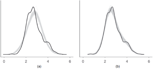
The model shown in the right panel (b) can simulate new data that are more
similar to the observed outcome than the model in the left panel (a). Thus,
model (b) is likely to be preferred over model (a).
Value
A data frame of simulated responses and the original response vector.
Note
Every model object that has a simulate()-method should work with
check_predictions(). On R 3.6.0 and higher, if bayesplot (or a
package that imports bayesplot such as rstanarm or brms)
is loaded, pp_check() is also available as an alias for check_predictions().
If check_predictions() doesn't work as expected, try setting verbose = TRUE
to get hints about possible problems.
References
Gabry, J., Simpson, D., Vehtari, A., Betancourt, M., and Gelman, A. (2019). Visualization in Bayesian workflow. Journal of the Royal Statistical Society: Series A (Statistics in Society), 182(2), 389–402. https://doi.org/10.1111/rssa.12378
Gelman, A., and Hill, J. (2007). Data analysis using regression and multilevel/hierarchical models. Cambridge; New York: Cambridge University Press.
Gelman, A., Carlin, J. B., Stern, H. S., Dunson, D. B., Vehtari, A., and Rubin, D. B. (2014). Bayesian data analysis. (Third edition). CRC Press.
Gelman, A., Hill, J., and Vehtari, A. (2020). Regression and Other Stories. Cambridge University Press.
See Also
simulate_residuals() and check_residuals(). See also
see::print.see_performance_pp_check() for options to customize the plot.
Other functions to check model assumptions and and assess model quality:
check_autocorrelation(),
check_collinearity(),
check_convergence(),
check_heteroscedasticity(),
check_homogeneity(),
check_model(),
check_outliers(),
check_overdispersion(),
check_singularity(),
check_zeroinflation()
Examples
# linear model
model <- lm(mpg ~ disp, data = mtcars)
check_predictions(model)

# discrete/integer outcome
set.seed(99)
d <- iris
d$skewed <- rpois(150, 1)
model <- glm(
  skewed ~ Species + Petal.Length + Petal.Width,
  family = poisson(),
  data = d
)
check_predictions(model, type = "discrete_both")
Check distribution of simulated quantile residuals
Description
check_residuals() checks generalized linear (mixed) models for uniformity
of randomized quantile residuals, which can be used to identify typical model
misspecification problems, such as over/underdispersion, zero-inflation, and
residual spatial and temporal autocorrelation.
Usage
check_residuals(x, ...)

## Default S3 method:
check_residuals(x, alternative = "two.sided", distribution = "punif", ...)
Arguments
x |
A supported model object or an object returned by
|
... |
Passed down to |
alternative |
A character string specifying the alternative hypothesis.
Can be one of |
distribution |
The distribution to compare the residuals against.
Can be (a) a character value giving a cumulative distribution function
(for example, |
Details
Simulated quantile residuals are generated by simulating a series of
values from a fitted model for each case, comparing the observed response
values to these simulations, and computing the empirical quantile of the
observed value in the distribution of simulated values. When the model is
correctly-specified, these quantile residuals will follow a uniform (flat)
distribution. check_residuals() tests the distribution of the quantile
residuals against the uniform distribution using a Kolmogorov-Smirnov test.
Essentially, comparing quantile residuals to the uniform distribution tests
whether the observed response values deviate from model expectations
(i.e., simulated values). In this sense, check_residuals() is similar to
posterior predictive checks with check_predictions().
There is a plot() method to visualize the distribution of quantile residuals
using a Q-Q plot. This plot can be interpreted in the same way as a Q-Q plot
for normality of residuals in linear regression.
If desired, a different theoretical distribution or a vector of numeric
values can be tested against using the distribution argument.
Value
The p-value of the test statistics.
Tests based on simulated residuals
For certain models, resp. model from certain families, tests like
check_zeroinflation() or check_overdispersion() are based on
simulated residuals. These are usually more accurate for such tests than
the traditionally used Pearson residuals. However, when simulating from more
complex models, such as mixed models or models with zero-inflation, there are
several important considerations. simulate_residuals() relies on
DHARMa::simulateResiduals(), and additional arguments specified in ...
are passed further down to that function. The defaults in DHARMa are set on
the most conservative option that works for all models. However, in many
cases, the help advises to use different settings in particular situations
or for particular models. It is recommended to read the 'Details' in
?DHARMa::simulateResiduals closely to understand the implications of the
simulation process and which arguments should be modified to get the most
accurate results.
See Also
simulate_residuals(), check_zeroinflation(),
check_overdispersion() and check_predictions(). See also
see::plot.see_performance_simres() for options to customize the plot.
Examples
dat <- DHARMa::createData(sampleSize = 100, overdispersion = 0.5, family = poisson())
m <- glm(observedResponse ~ Environment1, family = poisson(), data = dat)
res <- simulate_residuals(m)
check_residuals(res)
Check mixed models for boundary fits
Description
Check mixed models for boundary fits.
Usage
check_singularity(x, tolerance = 1e-05, ...)

## S3 method for class 'glmmTMB'
check_singularity(x, tolerance = 1e-05, check = "model", ...)
Arguments
x |
A mixed model. |
tolerance |
Indicates up to which value the convergence result is
accepted. The larger |
... |
Currently not used. |
check |
Indicates whether singularity check should be carried out for
the full model ( |
Details
If a model is "singular", this means that some dimensions of the variance-covariance matrix have been estimated as exactly zero. This often occurs for mixed models with complex random effects structures.
"While singular models are statistically well defined (it is theoretically sensible for the true maximum likelihood estimate to correspond to a singular fit), there are real concerns that (1) singular fits correspond to overfitted models that may have poor power; (2) chances of numerical problems and mis-convergence are higher for singular models (e.g. it may be computationally difficult to compute profile confidence intervals for such models); (3) standard inferential procedures such as Wald statistics and likelihood ratio tests may be inappropriate." (lme4 Reference Manual)
There is no gold-standard about how to deal with singularity and which random-effects specification to choose. Beside using fully Bayesian methods (with informative priors), proposals in a frequentist framework are:
avoid fitting overly complex models, such that the variance-covariance matrices can be estimated precisely enough (Matuschek et al. 2017)
use some form of model selection to choose a model that balances predictive accuracy and overfitting/type I error (Bates et al. 2015, Matuschek et al. 2017)
"keep it maximal", i.e. fit the most complex model consistent with the experimental design, removing only terms required to allow a non-singular fit (Barr et al. 2013)
since version 1.1.9, the glmmTMB package allows to use priors in a frequentist framework, too. One recommendation is to use a Gamma prior (Chung et al. 2013). The mean may vary from 1 to very large values (like
1e8), and the shape parameter should be set to a value of 2.5. You can thenupdate()your model with the specified prior. In glmmTMB, the code would look like this:# "model" is an object of class gmmmTMB prior <- data.frame( prior = "gamma(1, 2.5)", # mean can be 1, but even 1e8 class = "ranef" # for random effects ) model_with_priors <- update(model, priors = prior)
Large values for the mean parameter of the Gamma prior have no large impact on the random effects variances in terms of a "bias". Thus, if
1doesn't fix the singular fit, you can safely try larger values.
Note the different meaning between singularity and convergence: singularity indicates an issue with the "true" best estimate, i.e. whether the maximum likelihood estimation for the variance-covariance matrix of the random effects is positive definite or only semi-definite. Convergence is a question of whether we can assume that the numerical optimization has worked correctly or not.
Value
TRUE if the model fit is singular.
References
Bates D, Kliegl R, Vasishth S, Baayen H. Parsimonious Mixed Models. arXiv:1506.04967, June 2015.
Barr DJ, Levy R, Scheepers C, Tily HJ. Random effects structure for confirmatory hypothesis testing: Keep it maximal. Journal of Memory and Language, 68(3):255-278, April 2013.
Chung Y, Rabe-Hesketh S, Dorie V, Gelman A, and Liu J. 2013. "A Nondegenerate Penalized Likelihood Estimator for Variance Parameters in Multilevel Models." Psychometrika 78 (4): 685–709. doi:10.1007/s11336-013-9328-2
Matuschek H, Kliegl R, Vasishth S, Baayen H, Bates D. Balancing type I error and power in linear mixed models. Journal of Memory and Language, 94:305-315, 2017.
lme4 Reference Manual, https://cran.r-project.org/package=lme4
See Also
Other functions to check model assumptions and and assess model quality:
check_autocorrelation(),
check_collinearity(),
check_convergence(),
check_heteroscedasticity(),
check_homogeneity(),
check_model(),
check_outliers(),
check_overdispersion(),
check_predictions(),
check_zeroinflation()
Examples
data(sleepstudy, package = "lme4")
set.seed(123)
sleepstudy$mygrp <- sample(1:5, size = 180, replace = TRUE)
sleepstudy$mysubgrp <- NA
for (i in 1:5) {
  filter_group <- sleepstudy$mygrp == i
  sleepstudy$mysubgrp[filter_group] <-
    sample(1:30, size = sum(filter_group), replace = TRUE)
}

model <- lme4::lmer(
  Reaction ~ Days + (1 | mygrp / mysubgrp) + (1 | Subject),
  data = sleepstudy
)
# any singular fits?
check_singularity(model)
# singular fit for which particular random effects terms?
check_singularity(model, check = "terms")

## Not run:
# Fixing singularity issues using priors in glmmTMB
# Example taken from `vignette("priors", package = "glmmTMB")`
dat <- readRDS(system.file(
  "vignette_data",
  "gophertortoise.rds",
  package = "glmmTMB"
))
model <- glmmTMB::glmmTMB(
  shells ~ prev + offset(log(Area)) + factor(year) + (1 | Site),
  family = poisson,
  data = dat
)
# singular fit
check_singularity(model)

# impose Gamma prior on random effects parameters
prior <- data.frame(
  prior = "gamma(1, 2.5)", # mean can be 1, but even 1e8
  class = "ranef" # for random effects
)
model_with_priors <- update(model, priors = prior)
# no singular fit
check_singularity(model_with_priors)

## End(Not run)
Check model for violation of sphericity
Description
Check model for violation of sphericity. For Bartlett's Test of Sphericity (used for correlation matrices and factor analyses), see check_sphericity_bartlett.
Usage
check_sphericity(x, ...)
Arguments
x |
A model object. |
... |
Arguments passed to |
Value
Invisibly returns the p-values of the test statistics. A p-value < 0.05 indicates a violation of sphericity.
Examples
data(Soils, package = "carData")
soils.mod <- lm(
  cbind(pH, N, Dens, P, Ca, Mg, K, Na, Conduc) ~ Block + Contour * Depth,
  data = Soils
)

check_sphericity(Manova(soils.mod))
Check distribution symmetry
Description
Uses Hotelling and Solomons test of symmetry by testing if the standardized
nonparametric skew (\frac{(Mean - Median)}{SD}) is different than 0.
This is an underlying assumption of Wilcoxon signed-rank test.
Usage
check_symmetry(x, ...)
Arguments
x |
Model or numeric vector |
... |
Not used. |
Examples
V <- suppressWarnings(wilcox.test(mtcars$mpg))
check_symmetry(V)
Check for zero-inflation in count models
Description
check_zeroinflation() checks whether count models are
over- or underfitting zeros in the outcome.
Usage
check_zeroinflation(x, ...)

## Default S3 method:
check_zeroinflation(x, tolerance = 0.05, ...)

## S3 method for class 'performance_simres'
check_zeroinflation(x, tolerance = 0.1, alternative = "two.sided", ...)
Arguments
x |
Fitted model of class |
... |
Arguments passed down to |
tolerance |
The tolerance for the ratio of observed and predicted
zeros to considered as over- or underfitting zeros. A ratio
between 1 +/- |
alternative |
A character string specifying the alternative hypothesis.
Can be one of |
Details
If the amount of observed zeros is larger than the amount of predicted zeros, the model is underfitting zeros, which indicates a zero-inflation in the data. In such cases, it is recommended to use negative binomial or zero-inflated models.
In case of negative binomial models, models with zero-inflation component,
or hurdle models, the results from check_zeroinflation() are based on
simulate_residuals(), i.e. check_zeroinflation(simulate_residuals(model))
is internally called if necessary.
Value
A list with information about the amount of predicted and observed zeros in the outcome, as well as the ratio between these two values.
Tests based on simulated residuals
For certain models, resp. model from certain families, tests are based on
simulated residuals (see simulate_residuals()). These are usually more
accurate for testing such models than the traditionally used Pearson residuals.
However, when simulating from more complex models, such as mixed models or
models with zero-inflation, there are several important considerations.
Arguments specified in ... are passed to simulate_residuals(), which
relies on DHARMa::simulateResiduals() (and therefore, arguments in ...
are passed further down to DHARMa). The defaults in DHARMa are set on the
most conservative option that works for all models. However, in many cases,
the help advises to use different settings in particular situations or for
particular models. It is recommended to read the 'Details' in
?DHARMa::simulateResiduals closely to understand the implications of the
simulation process and which arguments should be modified to get the most
accurate results.
See Also
Other functions to check model assumptions and and assess model quality:
check_autocorrelation(),
check_collinearity(),
check_convergence(),
check_heteroscedasticity(),
check_homogeneity(),
check_model(),
check_outliers(),
check_overdispersion(),
check_predictions(),
check_singularity()
Examples
data(Salamanders, package = "glmmTMB")
m <- glm(count ~ spp + mined, family = poisson, data = Salamanders)
check_zeroinflation(m)

# for models with zero-inflation component, it's better to carry out
# the check for zero-inflation using simulated residuals
m <- glmmTMB::glmmTMB(
  count ~ spp + mined,
  ziformula = ~ mined + spp,
  family = poisson,
  data = Salamanders
)
res <- simulate_residuals(m)
check_zeroinflation(res)
Classify the distribution of a model-family using machine learning
Description
Classify the distribution of a model-family using machine learning
Details
The trained model to classify distributions, which is used by the
check_distribution() function.
Compare performance of different models
Description
compare_performance() computes indices of model
performance for different models at once and hence allows comparison of
indices across models.
Usage
compare_performance(
  ...,
  metrics = "all",
  rank = FALSE,
  estimator = "ML",
  verbose = TRUE
)
Arguments
... |
Multiple model objects (also of different classes). |
metrics |
Can be |
rank |
Logical, if |
estimator |
Only for linear models. Corresponds to the different
estimators for the standard deviation of the errors. If |
verbose |
Toggle warnings. |
Details
Model Weights
When information criteria (IC) are requested in metrics (i.e., any of "all",
"common", "AIC", "AICc", "BIC", "WAIC", or "LOOIC"), model
weights based on these criteria are also computed. For all IC except LOOIC,
weights are computed as w = exp(-0.5 * delta_ic) / sum(exp(-0.5 * delta_ic)),
where delta_ic is the difference between the model's IC value and the
smallest IC value in the model set (Burnham and Anderson, 2002).
For LOOIC, weights are computed as "stacking weights" using
loo::stacking_weights().
Ranking Models
When rank = TRUE, a new column Performance_Score is returned.
This score ranges from 0\
performance. Note that all score value do not necessarily sum up to 100\
Rather, calculation is based on normalizing all indices (i.e. rescaling
them to a range from 0 to 1), and taking the mean value of all indices for
each model. This is a rather quick heuristic, but might be helpful as
exploratory index.
In particular when models are of different types (e.g. mixed models,
classical linear models, logistic regression, ...), not all indices will be
computed for each model. In case where an index can't be calculated for a
specific model type, this model gets an NA value. All indices that
have any NAs are excluded from calculating the performance score.
There is a plot()-method for compare_performance(),
which creates a "spiderweb" plot, where the different indices are
normalized and larger values indicate better model performance.
Hence, points closer to the center indicate worse fit indices
(see online-documentation
for more details).
REML versus ML estimator
By default, estimator = "ML", which means that values from information
criteria (AIC, AICc, BIC) for specific model classes (like models from lme4)
are based on the ML-estimator, while the default behaviour of AIC() for
such classes is setting REML = TRUE. This default is intentional, because
comparing information criteria based on REML fits is usually not valid
(it might be useful, though, if all models share the same fixed effects -
however, this is usually not the case for nested models, which is a
prerequisite for the LRT). Set estimator = "REML" explicitly return the
same (AIC/...) values as from the defaults in AIC.merMod().
Value
A data frame with one row per model and one column per "index" (see
metrics).
Note
There is also a plot()-method implemented in the see-package.
References
Burnham, K. P., and Anderson, D. R. (2002). Model selection and multimodel inference: A practical information-theoretic approach (2nd ed.). Springer-Verlag. doi:10.1007/b97636
Examples
data(iris)
lm1 <- lm(Sepal.Length ~ Species, data = iris)
lm2 <- lm(Sepal.Length ~ Species + Petal.Length, data = iris)
lm3 <- lm(Sepal.Length ~ Species * Petal.Length, data = iris)
compare_performance(lm1, lm2, lm3)
compare_performance(lm1, lm2, lm3, rank = TRUE)

m1 <- lm(mpg ~ wt + cyl, data = mtcars)
m2 <- glm(vs ~ wt + mpg, data = mtcars, family = "binomial")
m3 <- lme4::lmer(Petal.Length ~ Sepal.Length + (1 | Species), data = iris)
compare_performance(m1, m2, m3)
Cronbach's Alpha for Items or Scales
Description
Compute various measures of internal consistencies for tests or
item-scales of questionnaires. cronbachs_alpha() calculates the Cronbach's
Alpha value for all variables in x. item_alpha() is an alias for
cronbachs_alpha().
Usage
cronbachs_alpha(x, ...)

item_alpha(x, ...)

## S3 method for class 'data.frame'
cronbachs_alpha(x, verbose = TRUE, ...)
Arguments
x |
A matrix or a data frame, or an object of class |
... |
Currently not used. |
verbose |
Toggle warnings and messages. |
Details
The Cronbach's Alpha value for x. A value closer to 1
indicates greater internal consistency, where usually following
rule of thumb is applied to interpret the results:
- α
< 0.5 is unacceptable,
0.5 < α < 0.6 is poor,
0.6 < α < 0.7 is questionable,
0.7 < α < 0.8 is acceptable,
and everything > 0.8 is good or excellent.
Value
The Cronbach's Alpha value for x.
Note
item_alpha() is an alias for cronbachs_alpha().
References
Bland, J. M., and Altman, D. G. Statistics notes: Cronbach's alpha. BMJ 1997;314:572. 10.1136/bmj.314.7080.572
Examples
data(mtcars)
x <- mtcars[, c("cyl", "gear", "carb", "hp")]
cronbachs_alpha(x)
Print tables in different output formats
Description
Prints tables (i.e. data frame) in different output formats.
Usage
## S3 method for class 'performance_model'
display(object, format = "markdown", digits = 2, caption = NULL, ...)

## S3 method for class 'performance_model'
print(x, digits = 3, layout = "horizontal", ...)

## S3 method for class 'performance_model'
print_md(
  x,
  digits = 2,
  caption = "Indices of model performance",
  layout = "horizontal",
  ...
)

## S3 method for class 'compare_performance'
print_md(
  x,
  digits = 2,
  caption = "Comparison of Model Performance Indices",
  layout = "horizontal",
  ...
)
Arguments
object, x |
An object returned by one of the package's function, for
example |
format |
String, indicating the output format. Can be |
digits |
Number of decimal places. |
caption |
Table caption as string. If |
... |
Arguments passed to other methods, e.g. |
layout |
Table layout (can be either |
Details
display() is useful when the table-output from functions, which is
usually printed as formatted text-table to console, should be formatted for
pretty table-rendering in markdown documents, or if knitted from rmarkdown
to PDF or Word files. See
vignette
for examples.
Value
A character vector. If format = "markdown", the return value
will be a character vector in markdown-table format.
Global Options to Customize Output when Printing
-
easystats_display_format:options(easystats_display_format = <value>)will set the default format for thedisplay()methods. Can be one of"markdown","html", or"tt".
Examples
model <- lm(mpg ~ wt + cyl, data = mtcars)
mp <- model_performance(model)
display(mp)
display(mp, digits = 3, ic_digits = 4)
Intraclass Correlation Coefficient (ICC)
Description
This function calculates the intraclass-correlation coefficient (ICC) -
sometimes also called variance partition coefficient (VPC) or
repeatability - for mixed effects models. The ICC can be calculated for all
models supported by insight::get_variance(). For models fitted with the
brms-package, icc() might fail due to the large variety of
models and families supported by the brms-package. In such cases, an
alternative to the ICC is the variance_decomposition(), which is based
on the posterior predictive distribution (see 'Details').
Usage
icc(
  model,
  by_group = FALSE,
  tolerance = 1e-05,
  ci = NULL,
  iterations = 100,
  ci_method = NULL,
  null_model = NULL,
  approximation = "lognormal",
  model_component = NULL,
  verbose = TRUE,
  ...
)

variance_decomposition(model, re_formula = NULL, robust = TRUE, ci = 0.95, ...)
Arguments
model |
A (Bayesian) mixed effects model. |
by_group |
Logical, if |
tolerance |
Tolerance for singularity check of random effects, to decide
whether to compute random effect variances or not. Indicates up to which
value the convergence result is accepted. The larger tolerance is, the
stricter the test will be. See |
ci |
Confidence resp. credible interval level. For |
iterations |
Number of bootstrap-replicates when computing confidence intervals for the ICC, R2, RMSE etc. |
ci_method |
Character string, indicating the bootstrap-method. Should
be |
null_model |
Optional, a null model to compute the random effect variances,
which is passed to |
approximation |
Character string, indicating the approximation method
for the distribution-specific (observation level, or residual) variance. Only
applies to non-Gaussian models. Can be |
model_component |
For models that can have a zero-inflation component,
specify for which component variances should be returned. If |
verbose |
Toggle warnings and messages. |
... |
Arguments passed down to |
re_formula |
Formula containing group-level effects to be considered in
the prediction. If |
robust |
Logical, if |
Details
Interpretation
The ICC can be interpreted as "the proportion of the variance explained by the grouping structure in the population". The grouping structure entails that measurements are organized into groups (e.g., test scores in a school can be grouped by classroom if there are multiple classrooms and each classroom was administered the same test) and ICC indexes how strongly measurements in the same group resemble each other. This index goes from 0, if the grouping conveys no information, to 1, if all observations in a group are identical (Gelman and Hill, 2007, p. 258). In other word, the ICC - sometimes conceptualized as the measurement repeatability - "can also be interpreted as the expected correlation between two randomly drawn units that are in the same group" (Hox 2010: 15), although this definition might not apply to mixed models with more complex random effects structures. The ICC can help determine whether a mixed model is even necessary: an ICC of zero (or very close to zero) means the observations within clusters are no more similar than observations from different clusters, and setting it as a random factor might not be necessary.
Difference with R2
The coefficient of determination R2 (that can be computed with r2())
quantifies the proportion of variance explained by a statistical model, but
its definition in mixed model is complex (hence, different methods to compute
a proxy exist). ICC is related to R2 because they are both ratios of
variance components. More precisely, R2 is the proportion of the explained
variance (of the full model), while the ICC is the proportion of explained
variance that can be attributed to the random effects. In simple cases, the
ICC corresponds to the difference between the conditional R2 and the
marginal R2 (see r2_nakagawa()).
Calculation
The ICC is calculated by dividing the random effect variance, σ2i, by the total variance, i.e. the sum of the random effect variance and the residual variance, σ2ε.
Adjusted and unadjusted ICC
icc() calculates an adjusted and an unadjusted ICC, which both take all
sources of uncertainty (i.e. of all random effects) into account. While
the adjusted ICC only relates to the random effects, the unadjusted ICC
also takes the fixed effects variances into account, more precisely, the
fixed effects variance is added to the denominator of the formula to
calculate the ICC (see Nakagawa et al. 2017). Typically, the adjusted
ICC is of interest when the analysis of random effects is of interest.
icc() returns a meaningful ICC also for more complex random effects
structures, like models with random slopes or nested design (more than two
levels) and is applicable for models with other distributions than Gaussian.
For more details on the computation of the variances, see
?insight::get_variance.
ICC for unconditional and conditional models
Usually, the ICC is calculated for the null model ("unconditional model"). However, according to Raudenbush and Bryk (2002) or Rabe-Hesketh and Skrondal (2012) it is also feasible to compute the ICC for full models with covariates ("conditional models") and compare how much, e.g., a level-2 variable explains the portion of variation in the grouping structure (random intercept).
ICC for specific group-levels
The proportion of variance for specific levels related to the overall model
can be computed by setting by_group = TRUE. The reported ICC is
the variance for each (random effect) group compared to the total
variance of the model. For mixed models with a simple random intercept,
this is identical to the classical (adjusted) ICC.
Variance decomposition for brms-models
If model is of class brmsfit, icc() might fail due to the large
variety of models and families supported by the brms package. In such
cases, variance_decomposition() is an alternative ICC measure. The function
calculates a variance decomposition based on the posterior predictive
distribution. In this case, first, the draws from the posterior predictive
distribution not conditioned on group-level terms
(posterior_predict(..., re_formula = NA)) are calculated as well as draws
from this distribution conditioned on all random effects (by default,
unless specified else in re_formula) are taken. Then, second, the variances
for each of these draws are calculated. The "ICC" is then the ratio between
these two variances. This is the recommended way to analyse
random-effect-variances for non-Gaussian models. It is then possible to
compare variances across models, also by specifying different group-level
terms via the re_formula-argument.
Sometimes, when the variance of the posterior predictive distribution is
very large, the variance ratio in the output makes no sense, e.g. because
it is negative. In such cases, it might help to use robust = TRUE.
Value
A list with two values, the adjusted ICC and the unadjusted ICC. For
variance_decomposition(), a list with two values, the decomposed
ICC as well as the credible intervals for this ICC.
Supported models and model families
The single variance components that are required to calculate the marginal
and conditional r-squared values are calculated using the insight::get_variance()
function. The results are validated against the solutions provided by
Nakagawa et al. (2017), in particular examples shown in the Supplement 2
of the paper. Other model families are validated against results from the
MuMIn package. This means that the r-squared values returned by r2_nakagawa()
should be accurate and reliable for following mixed models or model families:
Bernoulli (logistic) regression
Binomial regression (with other than binary outcomes)
Poisson and Quasi-Poisson regression
Negative binomial regression (including nbinom1, nbinom2 and nbinom12 families)
Gaussian regression (linear models)
Gamma regression
Tweedie regression
Beta regression
Ordered beta regression
Following model families are not yet validated, but should work:
Zero-inflated and hurdle models
Beta-binomial regression
Compound Poisson regression
Generalized Poisson regression
Log-normal regression
Skew-normal regression
Extracting variance components for models with zero-inflation part is not straightforward, because it is not definitely clear how the distribution-specific variance should be calculated. Therefore, it is recommended to carefully inspect the results, and probably validate against other models, e.g. Bayesian models (although results may be only roughly comparable).
Log-normal regressions (e.g. lognormal() family in glmmTMB or gaussian("log"))
often have a very low fixed effects variance (if they were calculated as
suggested by Nakagawa et al. 2017). This results in very low ICC or
r-squared values, which may not be meaningful.
References
Hox, J. J. (2010). Multilevel analysis: techniques and applications (2nd ed). New York: Routledge.
Nakagawa, S., Johnson, P. C. D., and Schielzeth, H. (2017). The coefficient of determination R2 and intra-class correlation coefficient from generalized linear mixed-effects models revisited and expanded. Journal of The Royal Society Interface, 14(134), 20170213.
Rabe-Hesketh, S., and Skrondal, A. (2012). Multilevel and longitudinal modeling using Stata (3rd ed). College Station, Tex: Stata Press Publication.
Raudenbush, S. W., and Bryk, A. S. (2002). Hierarchical linear models: applications and data analysis methods (2nd ed). Thousand Oaks: Sage Publications.
Examples
model <- lme4::lmer(Sepal.Length ~ Petal.Length + (1 | Species), data = iris)
icc(model)

# ICC for specific group-levels
data(sleepstudy, package = "lme4")
set.seed(12345)
sleepstudy$grp <- sample(1:5, size = 180, replace = TRUE)
sleepstudy$subgrp <- NA
for (i in 1:5) {
  filter_group <- sleepstudy$grp == i
  sleepstudy$subgrp[filter_group] <-
    sample(1:30, size = sum(filter_group), replace = TRUE)
}
model <- lme4::lmer(
  Reaction ~ Days + (1 | grp / subgrp) + (1 | Subject),
  data = sleepstudy
)
icc(model, by_group = TRUE)
Difficulty of Questionnaire Items
Description
Compute various measures of internal consistencies for tests or item-scales of questionnaires.
Usage
item_difficulty(x, maximum_value = NULL)
Arguments
x |
Depending on the function, |
maximum_value |
Numeric value, indicating the maximum value of an item.
If |
Details
Item difficutly of an item is defined as the quotient of the sum
actually achieved for this item of all and the maximum achievable score. This
function calculates the item difficulty, which should range between 0.2 and
0.8. Lower values are a signal for more difficult items, while higher values
close to one are a sign for easier items. The ideal value for item difficulty
is p + (1 - p) / 2, where p = 1 / max(x). In most cases, the ideal item
difficulty lies between 0.5 and 0.8.
Value
A data frame with three columns: The name(s) of the item(s), the item difficulties for each item, and the ideal item difficulty.
References
Bortz, J., and Döring, N. (2006). Quantitative Methoden der Datenerhebung. In J. Bortz and N. Döring, Forschungsmethoden und Evaluation. Springer: Berlin, Heidelberg: 137–293
Kelava A, Moosbrugger H (2020). Deskriptivstatistische Itemanalyse und Testwertbestimmung. In: Moosbrugger H, Kelava A, editors. Testtheorie und Fragebogenkonstruktion. Berlin, Heidelberg: Springer, 143–158
Examples
data(mtcars)
x <- mtcars[, c("cyl", "gear", "carb", "hp")]
item_difficulty(x)
Discrimination and Item-Total Correlation of Questionnaire Items
Description
Compute various measures of internal consistencies for tests or
item-scales of questionnaires. item_discrimination() calculates the
corrected item-total correlations for each item of x with the remaining
items. item_totalcor() by default calculates the item-total correlations
(without correction).
Usage
item_discrimination(x, standardize = FALSE, corrected = TRUE, verbose = TRUE)

item_totalcor(x, standardize = FALSE, corrected = FALSE, verbose = TRUE)
Arguments
x |
A matrix or a data frame. |
standardize |
Logical, if |
corrected |
Logical, if |
verbose |
Toggle warnings and messages. |
Details
item_totalcor() calculates the item-total correlations (without
correction). A positive item-total correlation indicates that an item
successfully aligns with the overall test, with higher values signifying a
better fit. Conversely, a value near zero suggests the item is not measuring
the intended construct, while a negative correlation is a major red flag that
the item is flawed, miskeyed, or measures the opposite of what is intended.
This means a positive correlation is desired, a zero correlation is
problematic, and a negative correlation requires immediate attention.
The standard item-total correlation has an inherent flaw: the score of the
item being analyzed is included in the total score. This inclusion can
artificially inflate the correlation coefficient, as an item will always
correlate with itself. The corrected item-total correlation, or item
discrimination, addresses this issue by calculating the correlation between
the score on a single item and the sum of the scores of all other items on
the scale. This is done with item_discrimination(). The absolute value of
the item discrimination indices should be above 0.2. An index between 0.2
and 0.4 is considered as "fair", while a satisfactory index ranges from
0.4 to 0.7. Items with low discrimination indices are often ambiguously
worded and should be examined. Items with negative indices should be examined
to determine why a negative value was obtained (e.g. reversed answer
categories regarding positive and negative poles - in such cases, use
datawizard::reverse() to reverse-code items in advance).
Interpretation of the Corrected Item-Total Correlation Values:
| Corrected Item-Total Correlation Value | Interpretation | Action |
| Above 0.40 | The item has a very good discrimination and is strongly related to the underlying construct. | Retain the item. |
| 0.30 to 0.39 | The item has good discrimination and contributes positively to the scale's internal consistency. | Retain the item. |
| 0.20 to 0.29 | The item has marginal discrimination. While not ideal, it may still be acceptable, especially in shorter scales or when measuring a very broad construct. | Consider revising the item for clarity or content. If other items have stronger correlations, this one might be a candidate for removal if the scale needs to be shortened. |
| Below 0.20 | The item has poor discrimination. It does not correlate well with the rest of the scale and may be measuring something else. Its inclusion is likely to decrease the overall reliability (e.g., Cronbach's Alpha) of the scale. | Revise the item substantially or, more likely, remove it from the scale. |
| Negative Value | The item is negatively related to the rest of the scale. This is a serious issue. | The item must be revised or removed. Check for scoring errors (e.g., a reverse-keyed item that wasn't properly recoded). |
item_discrimination() and item_totalcor() only differ in the default
value of the corrected argument. The former calculates the corrected
item-total correlations, while the latter calculates the item-total
correlations.
Value
A data frame with the item discrimination (corrected item-total correlations) for each item of the scale.
References
Kelava A, Moosbrugger H (2020). Deskriptivstatistische Itemanalyse und Testwertbestimmung. In: Moosbrugger H, Kelava A, editors. Testtheorie und Fragebogenkonstruktion. Berlin, Heidelberg: Springer, 143–158
Examples
data(mtcars)
x <- mtcars[, c("cyl", "gear", "carb", "hp")]
item_discrimination(x)
item_totalcor(x)
Mean Inter-Item-Correlation
Description
Compute various measures of internal consistencies for tests or item-scales of questionnaires.
Usage
item_intercor(x, method = "pearson")
Arguments
x |
A matrix as returned by the |
method |
Correlation computation method. May be one of |
Details
This function calculates a mean inter-item-correlation, i.e. a
correlation matrix of x will be computed (unless x is already a matrix
as returned by the cor() function) and the mean of the sum of all items'
correlation values is returned. Requires either a data frame or a computed
cor() object.
"Ideally, the average inter-item correlation for a set of items should be between 0.20 and 0.40, suggesting that while the items are reasonably homogeneous, they do contain sufficiently unique variance so as to not be isomorphic with each other. When values are lower than 0.20, then the items may not be representative of the same content domain. If values are higher than 0.40, the items may be only capturing a small bandwidth of the construct." (Piedmont 2014)
Value
The mean inter-item-correlation value for x.
References
Piedmont RL. 2014. Inter-item Correlations. In: Michalos AC (eds) Encyclopedia of Quality of Life and Well-Being Research. Dordrecht: Springer, 3303-3304. doi:10.1007/978-94-007-0753-5_1493
Examples
data(mtcars)
x <- mtcars[, c("cyl", "gear", "carb", "hp")]
item_intercor(x)
McDonald's Omega for Items or Scales
Description
This function computes McDonald's omega reliability coefficients
alongside Cronbach's alpha for a set of items or a scale. It acts as a
wrapper for the psych::omega() function. The aim is to make McDonald's
omega readily available and present it with the widely-known Cronbach's
alpha, allowing for a more complete understanding of scale reliability. The
output includes various forms of omega (e.g., total, hierarchical) depending
on the factor structure specified.
Usage
item_omega(x, ...)

## S3 method for class 'data.frame'
item_omega(
  x,
  n = "auto",
  rotation = "oblimin",
  factor_method = "minres",
  poly_cor = FALSE,
  verbose = TRUE,
  ...
)

## S3 method for class 'matrix'
item_omega(
  x,
  n = "auto",
  rotation = "oblimin",
  factor_method = "minres",
  n_obs = NULL,
  poly_cor = FALSE,
  verbose = TRUE,
  ...
)
Arguments
x |
A matrix or a data frame. |
... |
Additional arguments passed to |
n |
Number of factors to extract. |
rotation |
Rotation to be applied. Defaults to |
factor_method |
The factoring method to be used. Passed to the |
poly_cor |
Logical, if |
verbose |
Logical, if |
n_obs |
Number of observations in the original data set if |
Details
item_omega() is a simple wrapper around psych::omega(), which returns
the reliability coefficients. The original object returned by psych::omega()
is saved as $model attribute. Further information are accessible via the
summary() and parameters::model_parameters() methods. Use as.numeric()
to return the reliability coefficients as (named) numeric vector. Detailed
information can be found in the docs of ?psych::omega.
Value
A data frames containing the reliability coefficients. Use summary()
or parameters::model_parameters() on the returned object to extract more
information.
References
Bland, J. M., & Altman, D. G. (1997). Statistics notes: Cronbach's alpha. BMJ, 314(7080), 572. doi:10.1136/bmj.314.7080.572
Revelle, W., & Zinbarg, R. E. (2009). Coefficients alpha, beta, omega, and the glb: Comments on Sijtsma. Psychometrika, 74(1), 145–154. doi:10.1007/s11336-008-9102-z
Zinbarg, R.E., Revelle, W., Yovel, I., & Li. W. (2005). Cronbach's Alpha, Revelle's Beta, McDonald's Omega: Their relations with each and two alternative conceptualizations of reliability. Psychometrika. 70, 123-133
Examples
data(mtcars)
x <- mtcars[1:7]
result <- item_omega(x, n = 2)

result

as.numeric(result)

summary(result)

parameters::model_parameters(result)
Reliability Test for Items or Scales
Description
Compute various measures of internal consistencies for tests or item-scales of questionnaires.
Usage
item_reliability(x, standardize = FALSE, digits = 3, verbose = TRUE)
Arguments
x |
A matrix or a data frame. |
standardize |
Logical, if |
digits |
Amount of digits for returned values. |
verbose |
Toggle warnings and messages. |
Details
This function calculates the item-total correlations, item discriminations
(corrected item-total correlations for each item of x with the remaining
items) and the Cronbach's alpha for each item, if it was deleted from the
scale. The absolute value of the item discrimination indices should be above
0.2. An index between 0.2 and 0.4 is considered as "fair", while an index
above 0.4 (or below -0.4) is "good". The range of satisfactory values is from
0.4 to 0.7. Items with low discrimination indices are often ambiguously
worded and should be examined. Items with negative indices should be examined
to determine why a negative value was obtained (e.g. reversed answer
categories regarding positive and negative poles).
See check_itemscale() and item_discrimination() for more details on
the interpretation of the results.
Value
A data frame with the item-total correlations (column
Item_Total_Correlation), corrected item-total correlations (item
discrimination, column Discrimination) and Cronbach's Alpha (if item
deleted, column Alpha_if_deleted) for each item of the scale, or NULL if
data frame had too less columns.
Note
-
Item difficulty should range between 0.2 and 0.8. Ideal value is
p+(1-p)/2(which mostly is between 0.5 and 0.8). Seeitem_difficulty()for details. For item discrimination, also known as corrected item-total correlations, acceptable values are 0.20 or higher; the closer to 1.00 the better. See
item_discrimination()for more details. If an item discrimination is negative, the corresponding item probably need to be reverse-coded (which can be done withdatawizard::reverse()).In case the total Cronbach's alpha value is below the acceptable cut-off of 0.7 (mostly if an index has few items), the mean inter-item-correlation is an alternative measure to indicate acceptability. Satisfactory range lies between 0.2 and 0.4. See also
item_intercor().
References
Briggs SR, Cheek JM (1986) The role of factor analysis in the development and evaluation of personality scales. Journal of Personality, 54(1), 106-148. doi: 10.1111/j.1467-6494.1986.tb00391.x
Examples
data(mtcars)
x <- mtcars[, c("cyl", "gear", "carb", "hp")]
item_reliability(x)
Split-Half Reliability
Description
Compute various measures of internal consistencies for tests or item-scales of questionnaires.
Usage
item_split_half(x, digits = 3)
Arguments
x |
A matrix or a data frame. |
digits |
Amount of digits for returned values. |
Details
This function calculates the split-half reliability for items in
x, including the Spearman-Brown adjustment. Splitting is done by
selecting odd versus even columns in x. A value closer to 1
indicates greater internal consistency.
Value
A list with two elements: the split-half reliability splithalf
and the Spearman-Brown corrected split-half reliability
spearmanbrown.
References
Spearman C. 1910. Correlation calculated from faulty data. British Journal of Psychology (3): 271-295. doi:10.1111/j.2044-8295.1910.tb00206.x
Brown W. 1910. Some experimental results in the correlation of mental abilities. British Journal of Psychology (3): 296-322. doi:10.1111/j.2044-8295.1910.tb00207.x
Examples
data(mtcars)
x <- mtcars[, c("cyl", "gear", "carb", "hp")]
item_split_half(x)
LOO-related Indices for Bayesian regressions.
Description
Compute LOOIC (leave-one-out cross-validation (LOO) information criterion) and ELPD (expected log predictive density) for Bayesian regressions. For LOOIC and ELPD, smaller and larger values are respectively indicative of a better fit.
Usage
looic(model, verbose = TRUE)
Arguments
model |
A Bayesian regression model. |
verbose |
Toggle off warnings. |
Value
A list with four elements, the ELPD, LOOIC and their standard errors.
Examples
model <- suppressWarnings(rstanarm::stan_glm(
  mpg ~ wt + cyl,
  data = mtcars,
  chains = 1,
  iter = 500,
  refresh = 0
))
looic(model)
Model Performance
Description
See the documentation for your object's class:
Usage
model_performance(model, ...)

performance(model, ...)
Arguments
model |
Statistical model. |
... |
Arguments passed to or from other methods, resp. for
|
Details
model_performance() correctly detects transformed response and
returns the "corrected" AIC and BIC value on the original scale. To get back
to the original scale, the likelihood of the model is multiplied by the
Jacobian/derivative of the transformation.
Value
A data frame (with one row) and one column per "index" (see metrics).
See Also
compare_performance() to compare performance of many different models.
Examples
model <- lm(mpg ~ wt + cyl, data = mtcars)
model_performance(model)

model <- glm(vs ~ wt + mpg, data = mtcars, family = "binomial")
model_performance(model)
Performance of FA / PCA models
Description
Compute indices of model performance for models from the psych package,
and for parameters::factor_analysis() and item_omega().
Usage
## S3 method for class 'fa'
model_performance(model, metrics = "all", verbose = TRUE, ...)
Arguments
model |
A model object of class |
metrics |
Can be |
verbose |
Toggle off warnings. |
... |
Arguments passed to or from other methods. |
Details
The RMSR_corrected metric is the Root Mean Square Residual corrected for
degrees of freedom (i.e., dividing by degrees of freedom rather than the
number of observations).
For omega-models, the columns R2 and Correlation are measures of factor
score adequacy. R2 refers to the multiple R square of scores with factors,
while Correlation indicates the correlation of scores with factors.
Value
A data frame (with one row) and one column per "index" (see
metrics).
Examples
out <- psych::fa(psychTools::bfi[, 1:25], 5)
model_performance(out)

out <- item_omega(mtcars, n = 3)
model_performance(out)
Performance of instrumental variable regression models
Description
Performance of instrumental variable regression models
Usage
## S3 method for class 'ivreg'
model_performance(model, metrics = "all", verbose = TRUE, ...)
Arguments
model |
A model. |
metrics |
Can be |
verbose |
Toggle off warnings. |
... |
Arguments passed to or from other methods. |
Details
model_performance() correctly detects transformed response and
returns the "corrected" AIC and BIC value on the original scale. To get back
to the original scale, the likelihood of the model is multiplied by the
Jacobian/derivative of the transformation.
Model summary for k-means clustering
Description
Model summary for k-means clustering
Usage
## S3 method for class 'kmeans'
model_performance(model, verbose = TRUE, ...)
Arguments
model |
Object of type |
verbose |
Toggle off warnings. |
... |
Arguments passed to or from other methods. |
Examples
# a 2-dimensional example
x <- rbind(
  matrix(rnorm(100, sd = 0.3), ncol = 2),
  matrix(rnorm(100, mean = 1, sd = 0.3), ncol = 2)
)
colnames(x) <- c("x", "y")
model <- kmeans(x, 2)
model_performance(model)
Performance of lavaan SEM / CFA Models
Description
Compute indices of model performance for SEM or CFA models from the lavaan package.
Usage
## S3 method for class 'lavaan'
model_performance(model, metrics = "all", verbose = TRUE, ...)
Arguments
model |
A lavaan model. |
metrics |
Can be |
verbose |
Toggle off warnings. |
... |
Arguments passed to or from other methods. |
Details
Indices of fit
-
Chisq: The model Chi-squared assesses overall fit and the discrepancy between the sample and fitted covariance matrices. Its p-value should be > .05 (i.e., the hypothesis of a perfect fit cannot be rejected). However, it is quite sensitive to sample size.
-
GFI/AGFI: The (Adjusted) Goodness of Fit is the proportion of variance accounted for by the estimated population covariance. Analogous to R2. The GFI and the AGFI should be > .95 and > .90, respectively.
-
NFI/NNFI/TLI: The (Non) Normed Fit Index. An NFI of 0.95, indicates the model of interest improves the fit by 95\ null model. The NNFI (also called the Tucker Lewis index; TLI) is preferable for smaller samples. They should be > .90 (Byrne, 1994) or > .95 (Schumacker and Lomax, 2004).
-
CFI: The Comparative Fit Index is a revised form of NFI. Not very sensitive to sample size (Fan, Thompson, and Wang, 1999). Compares the fit of a target model to the fit of an independent, or null, model. It should be > .90.
-
RMSEA: The Root Mean Square Error of Approximation is a parsimony-adjusted index. Values closer to 0 represent a good fit. It should be < .08 or < .05. The p-value printed with it tests the hypothesis that RMSEA is less than or equal to .05 (a cutoff sometimes used for good fit), and thus should be not significant.
-
RMR/SRMR: the (Standardized) Root Mean Square Residual represents the square-root of the difference between the residuals of the sample covariance matrix and the hypothesized model. As the RMR can be sometimes hard to interpret, better to use SRMR. Should be < .08.
-
RFI: the Relative Fit Index, also known as RHO1, is not guaranteed to vary from 0 to 1. However, RFI close to 1 indicates a good fit.
-
IFI: the Incremental Fit Index (IFI) adjusts the Normed Fit Index (NFI) for sample size and degrees of freedom (Bollen's, 1989). Over 0.90 is a good fit, but the index can exceed 1.
-
PNFI: the Parsimony-Adjusted Measures Index. There is no commonly agreed-upon cutoff value for an acceptable model for this index. Should be > 0.50.
See the documentation for ?lavaan::fitmeasures.
What to report
Kline (2015) suggests that at a minimum the following indices should be reported: The model chi-square, the RMSEA, the CFI and the SRMR.
Value
A data frame (with one row) and one column per "index" (see
metrics).
References
Byrne, B. M. (1994). Structural equation modeling with EQS and EQS/Windows. Thousand Oaks, CA: Sage Publications.
Tucker, L. R., and Lewis, C. (1973). The reliability coefficient for maximum likelihood factor analysis. Psychometrika, 38, 1-10.
Schumacker, R. E., and Lomax, R. G. (2004). A beginner's guide to structural equation modeling, Second edition. Mahwah, NJ: Lawrence Erlbaum Associates.
Fan, X., B. Thompson, and L. Wang (1999). Effects of sample size, estimation method, and model specification on structural equation modeling fit indexes. Structural Equation Modeling, 6, 56-83.
Kline, R. B. (2015). Principles and practice of structural equation modeling. Guilford publications.
Examples
# Confirmatory Factor Analysis (CFA) ---------
data(HolzingerSwineford1939, package = "lavaan")
structure <- " visual  =~ x1 + x2 + x3
               textual =~ x4 + x5 + x6
               speed   =~ x7 + x8 + x9 "
model <- lavaan::cfa(structure, data = HolzingerSwineford1939)
model_performance(model)
Performance of Regression Models
Description
Compute indices of model performance for regression models.
Usage
## S3 method for class 'lm'
model_performance(model, metrics = "all", verbose = TRUE, ...)
Arguments
model |
A model. |
metrics |
Can be |
verbose |
Toggle off warnings. |
... |
Arguments passed to or from other methods. |
Details
Depending on model, following indices are computed:
-
AIC: Akaike's Information Criterion, see
?stats::AIC -
AICc: Second-order (or small sample) AIC with a correction for small sample sizes
-
BIC: Bayesian Information Criterion, see
?stats::BIC -
R2: r-squared value, see
r2() -
R2_adj: adjusted r-squared, see
r2() -
RMSE: root mean squared error, see
performance_rmse() -
SIGMA: residual standard deviation, see
insight::get_sigma() -
LOGLOSS: Log-loss, see
performance_logloss() -
SCORE_LOG: score of logarithmic proper scoring rule, see
performance_score() -
SCORE_SPHERICAL: score of spherical proper scoring rule, see
performance_score() -
PCP: percentage of correct predictions, see
performance_pcp()
model_performance() correctly detects transformed response and
returns the "corrected" AIC and BIC value on the original scale. To get back
to the original scale, the likelihood of the model is multiplied by the
Jacobian/derivative of the transformation.
Value
A data frame (with one row) and one column per "index" (see metrics).
Examples
model <- lm(mpg ~ wt + cyl, data = mtcars)
model_performance(model)

model <- glm(vs ~ wt + mpg, data = mtcars, family = "binomial")
model_performance(model)
Performance of Mixed Models
Description
Compute indices of model performance for mixed models.
Usage
## S3 method for class 'merMod'
model_performance(
  model,
  metrics = "all",
  estimator = "REML",
  verbose = TRUE,
  ...
)
Arguments
model |
A mixed effects model. |
metrics |
Can be |
estimator |
Only for linear models. Corresponds to the different
estimators for the standard deviation of the errors. If |
verbose |
Toggle warnings and messages. |
... |
Arguments passed to or from other methods. |
Details
Intraclass Correlation Coefficient (ICC)
This method returns the adjusted ICC only, as this is typically of
interest when judging the variance attributed to the random effects part of
the model (see also icc()).
REML versus ML estimator
The default behaviour of model_performance() when computing AIC or BIC of
linear mixed model from package lme4 is the same as for AIC() or
BIC() (i.e. estimator = "REML"). However, for model comparison using
compare_performance() sets estimator = "ML" by default, because
comparing information criteria based on REML fits is usually not valid
(unless all models have the same fixed effects). Thus, make sure to set
the correct estimator-value when looking at fit-indices or comparing model
fits.
Other performance indices
Furthermore, see 'Details' in model_performance.lm() for more details
on returned indices.
Value
A data frame (with one row) and one column per "index" (see
metrics).
Examples
model <- lme4::lmer(Petal.Length ~ Sepal.Length + (1 | Species), data = iris)
model_performance(model)
Performance of Meta-Analysis Models
Description
Compute indices of model performance for meta-analysis model from the metafor package.
Usage
## S3 method for class 'rma'
model_performance(
  model,
  metrics = "all",
  estimator = "ML",
  verbose = TRUE,
  ...
)
Arguments
model |
A |
metrics |
Can be |
estimator |
Only for linear models. Corresponds to the different
estimators for the standard deviation of the errors. If |
verbose |
Toggle off warnings. |
... |
Arguments passed to or from other methods. |
Details
Indices of fit
-
AIC Akaike's Information Criterion, see
?stats::AIC -
BIC Bayesian Information Criterion, see
?stats::BIC -
I2: For a random effects model,
I2estimates (in percent) how much of the total variability in the effect size estimates can be attributed to heterogeneity among the true effects. For a mixed-effects model,I2estimates how much of the unaccounted variability can be attributed to residual heterogeneity. -
H2: For a random-effects model,
H2estimates the ratio of the total amount of variability in the effect size estimates to the amount of sampling variability. For a mixed-effects model,H2estimates the ratio of the unaccounted variability in the effect size estimates to the amount of sampling variability. -
TAU2: The amount of (residual) heterogeneity in the random or mixed effects model.
-
CochransQ (QE): Test for (residual) Heterogeneity. Without moderators in the model, this is simply Cochran's Q-test.
-
Omnibus (QM): Omnibus test of parameters.
-
R2: Pseudo-R2-statistic, which indicates the amount of heterogeneity accounted for by the moderators included in a fixed-effects model.
See the documentation for ?metafor::fitstats.
Value
A data frame (with one row) and one column per "index" (see
metrics).
Examples
data(dat.bcg, package = "metadat")
dat <- metafor::escalc(
  measure = "RR",
  ai = tpos,
  bi = tneg,
  ci = cpos,
  di = cneg,
  data = dat.bcg
)
model <- metafor::rma(yi, vi, data = dat, method = "REML")
model_performance(model)
Performance of Bayesian Models
Description
Compute indices of model performance for (general) linear models.
Usage
## S3 method for class 'stanreg'
model_performance(model, metrics = "all", verbose = TRUE, ...)

## S3 method for class 'BFBayesFactor'
model_performance(
  model,
  metrics = "all",
  verbose = TRUE,
  average = FALSE,
  prior_odds = NULL,
  ...
)
Arguments
model |
Object of class |
metrics |
Can be |
verbose |
Toggle off warnings. |
... |
Arguments passed to or from other methods. |
average |
Compute model-averaged index? See |
prior_odds |
Optional vector of prior odds for the models compared to
the first model (or the denominator, for |
Details
Depending on model, the following indices are computed:
-
ELPD: expected log predictive density. Larger ELPD values mean better fit. See
looic(). -
LOOIC: leave-one-out cross-validation (LOO) information criterion. Lower LOOIC values mean better fit. See
looic(). -
WAIC: widely applicable information criterion. Lower WAIC values mean better fit. See
?loo::waic. -
R2: r-squared value, see
r2_bayes(). -
R2_adjusted: LOO-adjusted r-squared, see
r2_loo(). -
RMSE: root mean squared error, see
performance_rmse(). -
SIGMA: residual standard deviation, see
insight::get_sigma(). -
LOGLOSS: Log-loss, see
performance_logloss(). -
SCORE_LOG: score of logarithmic proper scoring rule, see
performance_score(). -
SCORE_SPHERICAL: score of spherical proper scoring rule, see
performance_score(). -
PCP: percentage of correct predictions, see
performance_pcp().
Value
A data frame (with one row) and one column per "index" (see
metrics).
References
Gelman, A., Goodrich, B., Gabry, J., and Vehtari, A. (2018). R-squared for Bayesian regression models. The American Statistician, The American Statistician, 1-6.
See Also
Examples
model <- suppressWarnings(rstanarm::stan_glm(
  mpg ~ wt + cyl,
  data = mtcars,
  chains = 1,
  iter = 500,
  refresh = 0
))
model_performance(model)

model <- suppressWarnings(rstanarm::stan_glmer(
  mpg ~ wt + cyl + (1 | gear),
  data = mtcars,
  chains = 1,
  iter = 500,
  refresh = 0
))
model_performance(model)
Accuracy of predictions from model fit
Description
This function calculates the predictive accuracy of linear or logistic regression models.
Usage
performance_accuracy(
  model,
  method = "cv",
  k = 5,
  n = 1000,
  ci = 0.95,
  verbose = TRUE
)
Arguments
model |
A linear or logistic regression model. A mixed-effects model is also accepted. |
method |
Character string, indicating whether cross-validation
( |
k |
The number of folds for the k-fold cross-validation. |
n |
Number of bootstrap-samples. |
ci |
The level of the confidence interval. |
verbose |
Toggle warnings. |
Details
For linear models, the accuracy is the correlation coefficient
between the actual and the predicted value of the outcome. For logistic
regression models, the accuracy corresponds to the AUC-value, calculated with
the bayestestR::auc()-function.
The accuracy is the mean value of multiple correlation resp. AUC-values,
which are either computed with cross-validation or non-parametric
bootstrapping (see argument method). The standard error is the standard
deviation of the computed correlation resp. AUC-values.
Value
A list with three values: The Accuracy of the model predictions,
i.e. the proportion of accurately predicted values from the model, its
standard error, SE, and the Method used to compute the accuracy.
Examples
model <- lm(mpg ~ wt + cyl, data = mtcars)
performance_accuracy(model)

model <- glm(vs ~ wt + mpg, data = mtcars, family = "binomial")
performance_accuracy(model)
Compute the AIC or second-order AIC
Description
Compute the AIC or the second-order Akaike's information criterion (AICc).
performance_aic() is a small wrapper that returns the AIC, however, for
models with a transformed response variable, performance_aic() returns the
corrected AIC value (see 'Examples'). It is a generic function that also
works for some models that don't have a AIC method (like Tweedie models).
performance_aicc() returns the second-order (or "small sample") AIC that
incorporates a correction for small sample sizes.
Usage
performance_aicc(x, ...)

performance_aic(x, ...)

## Default S3 method:
performance_aic(x, estimator = "ML", verbose = TRUE, ...)

## S3 method for class 'lmerMod'
performance_aic(x, estimator = "REML", verbose = TRUE, ...)
Arguments
x |
A model object. |
... |
Currently not used. |
estimator |
Only for linear models. Corresponds to the different
estimators for the standard deviation of the errors. If |
verbose |
Toggle warnings. |
Details
performance_aic() correctly detects transformed response and,
unlike stats::AIC(), returns the "corrected" AIC value on the original
scale. To get back to the original scale, the likelihood of the model is
multiplied by the Jacobian/derivative of the transformation.
In case it is not possible to return the corrected AIC value, a warning is given that the corrected log-likelihood value could not be computed.
Value
Numeric, the AIC or AICc value.
References
Akaike, H. (1973) Information theory as an extension of the maximum likelihood principle. In: Second International Symposium on Information Theory, pp. 267-281. Petrov, B.N., Csaki, F., Eds, Akademiai Kiado, Budapest.
Hurvich, C. M., Tsai, C.-L. (1991) Bias of the corrected AIC criterion for underfitted regression and time series models. Biometrika 78, 499–509.
Examples
m <- lm(mpg ~ wt + cyl + gear + disp, data = mtcars)
AIC(m)
performance_aicc(m)

# correct AIC for models with transformed response variable
data("mtcars")
mtcars$mpg <- floor(mtcars$mpg)
model <- lm(log(mpg) ~ factor(cyl), mtcars)

# wrong AIC, not corrected for log-transformation
AIC(model)

# performance_aic() correctly detects transformed response and
# returns corrected AIC
performance_aic(model)

## Not run:
# there are a few exceptions where the corrected log-likelihood values
# cannot be returned. The following exampe gives a warning.
model <- lm(1 / mpg ~ factor(cyl), mtcars)
performance_aic(model)

## End(Not run)
Cross-validated model performance
Description
This function cross-validates regression models in a user-supplied new sample or by using holdout (train-test), k-fold, or leave-one-out cross-validation.
Usage
performance_cv(
  model,
  data = NULL,
  method = "holdout",
  metrics = "all",
  prop = 0.3,
  k = 5,
  stack = TRUE,
  verbose = TRUE,
  ...
)
Arguments
model |
A regression model. |
data |
Optional. A data frame containing the same variables as |
method |
Character string, indicating the cross-validation method to use:
whether holdout ( |
metrics |
Can be |
prop |
If |
k |
If |
stack |
Logical. If |
verbose |
Toggle warnings. |
... |
Not used. |
Value
A data frame with columns for each metric requested, as well as k
if method = "holdout" and the Method used for cross-validation. If
method = "holdout" and stack = TRUE, the standard error (standard
deviation across holdout folds) for each metric is also included.
Examples
model <- lm(mpg ~ wt + cyl, data = mtcars)
performance_cv(model)
Hosmer-Lemeshow goodness-of-fit test
Description
Check model quality of logistic regression models.
Usage
performance_hosmer(model, n_bins = 10)
Arguments
model |
A |
n_bins |
Numeric, the number of bins to divide the data. |
Details
A well-fitting model shows no significant difference between the model and the observed data, i.e. the reported p-value should be greater than 0.05.
Value
An object of class hoslem_test with following values:
chisq, the Hosmer-Lemeshow chi-squared statistic; df, degrees
of freedom and p.value the p-value for the goodness-of-fit test.
References
Hosmer, D. W., and Lemeshow, S. (2000). Applied Logistic Regression. Hoboken, NJ, USA: John Wiley and Sons, Inc. doi:10.1002/0471722146
Examples
model <- glm(vs ~ wt + mpg, data = mtcars, family = "binomial")
performance_hosmer(model)
Log Loss
Description
Compute the log loss for models with binary outcome.
Usage
performance_logloss(model, verbose = TRUE, ...)
Arguments
model |
Model with binary outcome. |
verbose |
Toggle off warnings. |
... |
Currently not used. |
Details
Logistic regression models predict the probability of an outcome of being a
"success" or "failure" (or 1 and 0 etc.). performance_logloss() evaluates
how good or bad the predicted probabilities are. High values indicate bad
predictions, while low values indicate good predictions. The lower the
log-loss, the better the model predicts the outcome.
Value
Numeric, the log loss of model.
See Also
Examples
data(mtcars)
m <- glm(formula = vs ~ hp + wt, family = binomial, data = mtcars)
performance_logloss(m)
Mean Absolute Error of Models
Description
Compute mean absolute error of models.
Usage
performance_mae(model, ...)

mae(model, ...)
Arguments
model |
A model. |
... |
Arguments passed down to |
Value
Numeric, the mean absolute error of model.
Examples
data(mtcars)
m <- lm(mpg ~ hp + gear, data = mtcars)
performance_mae(m)
Mean Square Error of Linear Models
Description
Compute mean square error of linear models.
Usage
performance_mse(model, ...)

mse(model, ...)
Arguments
model |
A model. |
... |
Arguments passed down to |
Details
The mean square error is the mean of the sum of squared residuals, i.e. it measures the average of the squares of the errors. Less technically speaking, the mean square error can be considered as the variance of the residuals, i.e. the variation in the outcome the model doesn't explain. Lower values (closer to zero) indicate better fit.
Value
Numeric, the mean square error of model.
Examples
data(mtcars)
m <- lm(mpg ~ hp + gear, data = mtcars)
performance_mse(m)
Percentage of Correct Predictions
Description
Percentage of correct predictions (PCP) for models with binary outcome.
Usage
performance_pcp(model, ci = 0.95, method = "Herron", verbose = TRUE)
Arguments
model |
Model with binary outcome. |
ci |
The level of the confidence interval. |
method |
Name of the method to calculate the PCP (see 'Details').
Default is |
verbose |
Toggle off warnings. |
Details
method = "Gelman-Hill" (or "gelman_hill") computes the
PCP based on the proposal from Gelman and Hill 2017, 99, which is
defined as the proportion of cases for which the deterministic prediction
is wrong, i.e. the proportion where the predicted probability is above 0.5,
although y=0 (and vice versa) (see also Herron 1999, 90).
method = "Herron" (or "herron") computes a modified version
of the PCP (Herron 1999, 90-92), which is the sum of predicted
probabilities, where y=1, plus the sum of 1 - predicted probabilities,
where y=0, divided by the number of observations. This approach is said to
be more accurate.
The PCP ranges from 0 to 1, where values closer to 1 mean that the model predicts the outcome better than models with an PCP closer to 0. In general, the PCP should be above 0.5 (i.e. 50\ Furthermore, the PCP of the full model should be considerably above the null model's PCP.
The likelihood-ratio test indicates whether the model has a significantly better fit than the null-model (in such cases, p < 0.05).
Value
A list with several elements: the percentage of correct predictions of the full and the null model, their confidence intervals, as well as the chi-squared and p-value from the Likelihood-Ratio-Test between the full and null model.
References
Herron, M. (1999). Postestimation Uncertainty in Limited Dependent Variable Models. Political Analysis, 8, 83–98.
Gelman, A., and Hill, J. (2007). Data analysis using regression and multilevel/hierarchical models. Cambridge; New York: Cambridge University Press, 99.
Examples
data(mtcars)
m <- glm(formula = vs ~ hp + wt, family = binomial, data = mtcars)
performance_pcp(m)
performance_pcp(m, method = "Gelman-Hill")
Random Effects Reliability
Description
These functions provide information about the reliability of group-level estimates (i.e., random effects) in mixed models. They are useful to assess whether the predictors yield consistent group-level variability. "Group-level" can refer, for instance, to different participants in a study, and the predictors to the effect of some experimental condition.
The conceptually related functions are implemented,
performance_reliability(), based on Rouder & Mehrvarz (2024) that uses
estimated model variances, and performance_dvour() (d-vour), which
corresponds to the Variability-Over-Uncertainty Ratio ("vour") between random
effects coefficient variability and their associated uncertainty.
Note: performance_reliability() requires to recompute the model to
estimate some of the variances of interest, which does not make it very
usable with Bayesian models. Please get in touch if you have would like to
help addressing this.
Usage
performance_reliability(x, ...)

performance_dvour(x, ...)
Arguments
x |
A model object. |
... |
Currently not used. |
Details
Reliability (Signal-to-Noise Ratio)
performance_reliability() estimates the reliability of random effects
(intercepts and slopes) in mixed-effects models using variance decomposition.
This method follows the hierarchical modeling framework of Rouder &
Mehrvarz (2024), defining reliability as the signal-to-noise variance
ratio:
\gamma^2 = \frac{\sigma_B^2}{\sigma_B^2 + \sigma_W^2}
where:
-
\sigma_B^2is the between-subject variance (i.e., variability across groups). -
\sigma_W^2is the within-subject variance (i.e., trial-level measurement noise).
This metric quantifies how much observed variability is due to actual differences between groups, rather than measurement error or within-group fluctuations.
To account for trial count (L), reliability is adjusted following:
E(r) = \frac{\gamma^2}{\gamma^2 + 1/L}
where L is the number of observations per random effect level (note
that Rouder (2024) recommends 2/L to adjust for contrast effects).
Variability-Over-Uncertainty Ratio (d-vour)
performance_dvour() computes an alternative reliability measure corresponding
to the normalized ratio of observed variability to uncertainty in random effect
estimates. This is defined as:
\text{D-vour} = \frac{\sigma_B^2}{\sigma_B^2 + \mu_{\text{SE}}^2}
where:
-
\sigma_B^2is the between-group variability (computed as the SD of the random effect estimates). -
\mu_{\text{SE}}^2is the mean squared uncertainty in random effect estimates (i.e., the average uncertainty).
Interpretation:
-
D-vour > 0.75: Strong group-level effects (between-group variance is at least 3 times greater than uncertainty).
-
D-vour ~ 0.5: Within-group and between-group variability are similar; random effect estimates should be used with caution.
-
D-vour < 0.5: Measurement noise dominates; random effect estimates are probably unreliable.
While d-vour shares some similarity to Rouder's Reliability, it does not explicitly model within-group trial-level noise and is only based on the random effect estimates, and can thus be not accurate when there is not a lot of random factor groups (the reliability of this index - the meta-reliability - depends on the number of groups).
References
Rouder, J. N., Pena, A. L., Mehrvarz, M., & Vandekerckhove, J. (2024). On Cronbach’s merger: Why experiments may not be suitable for measuring individual differences.
Rouder, J. N., & Mehrvarz, M. (2024). Hierarchical-model insights for planning and interpreting individual-difference studies of cognitive abilities. Current Directions in Psychological Science, 33(2), 128-135.
Williams, D. R., Mulder, J., Rouder, J. N., & Rast, P. (2021). Beneath the surface: Unearthing within-person variability and mean relations with Bayesian mixed models. Psychological methods, 26(1), 74.
Williams, D. R., Martin, S. R., DeBolt, M., Oakes, L., & Rast, P. (2020). A fine-tooth comb for measurement reliability: Predicting true score and error variance in hierarchical models.
Examples
url <- "https://raw.githubusercontent.com/easystats/circus/refs/heads/main/data/illusiongame.csv"
df <- read.csv(url)

m <- lme4::lmer(RT ~ (1 | Participant), data = df)
performance_reliability(m)
performance_dvour(m)

m <- glmmTMB::glmmTMB(RT ~ (1 | Participant), data = df)
performance_reliability(m)
performance_dvour(m)

m <- lme4::lmer(RT ~ (1 | Participant) + (1 | Trial), data = df)
performance_reliability(m)
performance_dvour(m)

m <- glmmTMB::glmmTMB(RT ~ (1 | Participant) + (1 | Trial), data = df)
performance_reliability(m)
performance_dvour(m)


m <- lme4::lmer(
  RT ~ Illusion_Difference + (Illusion_Difference | Participant) + (1 | Trial),
  data = df
)
performance_reliability(m)
performance_dvour(m)

m <- glmmTMB::glmmTMB(
  RT ~ Illusion_Difference + (Illusion_Difference | Participant) + (1 | Trial),
  data = df
)
performance_reliability(m)
performance_dvour(m)
Root Mean Squared Error
Description
Compute root mean squared error for (mixed effects) models, including Bayesian regression models.
Usage
performance_rmse(
  model,
  normalized = FALSE,
  ci = NULL,
  iterations = 100,
  ci_method = NULL,
  verbose = TRUE,
  ...
)

rmse(
  model,
  normalized = FALSE,
  ci = NULL,
  iterations = 100,
  ci_method = NULL,
  verbose = TRUE,
  ...
)
Arguments
model |
A model. |
normalized |
Logical, use |
ci |
Confidence resp. credible interval level. For |
iterations |
Number of bootstrap-replicates when computing confidence intervals for the ICC, R2, RMSE etc. |
ci_method |
Character string, indicating the bootstrap-method. Should
be |
verbose |
Toggle warnings and messages. |
... |
Arguments passed down to |
Details
The RMSE is the square root of the variance of the residuals and indicates the absolute fit of the model to the data (difference between observed data to model's predicted values). It can be interpreted as the standard deviation of the unexplained variance, and is in the same units as the response variable. Lower values indicate better model fit.
The normalized RMSE is the proportion of the RMSE related to the range of the response variable. Hence, lower values indicate less residual variance.
Value
Numeric, the root mean squared error.
Examples
data(Orthodont, package = "nlme")
m <- nlme::lme(distance ~ age, data = Orthodont)

# RMSE
performance_rmse(m, normalized = FALSE)

# normalized RMSE
performance_rmse(m, normalized = TRUE)
Simple ROC curve
Description
This function calculates a simple ROC curves of x/y coordinates based on response and predictions of a binomial model.
It returns the area under the curve (AUC) as a percentage, which corresponds to the probability that a randomly chosen observation of "condition 1" is correctly classified by the model as having a higher probability of being "condition 1" than a randomly chosen "condition 2" observation.
Applying as.data.frame() to the output returns a data frame containing the
following:
-
Sensitivity(that actually corresponds to1 - Specificity): It is the False Positive Rate. -
Sensitivity: It is the True Positive Rate, which is the proportion of correctly classified "condition 1" observations.
Usage
performance_roc(x, ..., predictions, new_data)
Arguments
x |
A numeric vector, representing the outcome (0/1), or a model with binomial outcome. |
... |
One or more models with binomial outcome. In this case,
|
predictions |
If |
new_data |
If |
Value
A data frame with three columns, the x/y-coordinate pairs for the ROC
curve (Sensitivity and Specificity), and a column with the
model name.
Note
There is also a plot()-method
implemented in the see-package.
Examples
library(bayestestR)
data(iris)

set.seed(123)
iris$y <- rbinom(nrow(iris), size = 1, .3)
folds <- sample(nrow(iris), size = nrow(iris) / 8, replace = FALSE)
test_data <- iris[folds, ]
train_data <- iris[-folds, ]

model <- glm(y ~ Sepal.Length + Sepal.Width, data = train_data, family = "binomial")
as.data.frame(performance_roc(model, new_data = test_data))
as.numeric(performance_roc(model))

roc <- performance_roc(model, new_data = test_data)
area_under_curve(roc$Specificity, roc$Sensitivity)

if (interactive()) {
  m1 <- glm(y ~ Sepal.Length + Sepal.Width, data = iris, family = "binomial")
  m2 <- glm(y ~ Sepal.Length + Petal.Width, data = iris, family = "binomial")
  m3 <- glm(y ~ Sepal.Length + Species, data = iris, family = "binomial")
  performance_roc(m1, m2, m3)

  # if you have `see` package installed, you can also plot comparison of
  # ROC curves for different models
  if (require("see")) plot(performance_roc(m1, m2, m3))
}
Residual Standard Error for Linear Models
Description
Compute residual standard error of linear models.
Usage
performance_rse(model)
Arguments
model |
A model. |
Details
The residual standard error is the square root of the residual sum of squares divided by the residual degrees of freedom.
Value
Numeric, the residual standard error of model.
Examples
data(mtcars)
m <- lm(mpg ~ hp + gear, data = mtcars)
performance_rse(m)
Proper Scoring Rules
Description
Calculates the logarithmic, quadratic/Brier and spherical score from a model with binary or count outcome.
Usage
performance_score(model, verbose = TRUE, ...)
Arguments
model |
Model with binary or count outcome. |
verbose |
Toggle off warnings. |
... |
Arguments from other functions, usually only used internally. |
Details
Proper scoring rules can be used to evaluate the quality of model
predictions and model fit. performance_score() calculates the logarithmic,
quadratic/Brier and spherical scoring rules. The spherical rule takes values
in the interval [0, 1], with values closer to 1 indicating a more
accurate model, and the logarithmic rule in the interval [-Inf, 0],
with values closer to 0 indicating a more accurate model.
For stan_lmer() and stan_glmer() models, the predicted values
are based on posterior_predict(), instead of predict(). Thus,
results may differ more than expected from their non-Bayesian counterparts
in lme4.
Value
A list with three elements, the logarithmic, quadratic/Brier and spherical score.
Note
Code is partially based on GLMMadaptive::scoring_rules().
References
Carvalho, A. (2016). An overview of applications of proper scoring rules. Decision Analysis 13, 223–242. doi:10.1287/deca.2016.0337
See Also
Examples
## Dobson (1990) Page 93: Randomized Controlled Trial :
counts <- c(18, 17, 15, 20, 10, 20, 25, 13, 12)
outcome <- gl(3, 1, 9)
treatment <- gl(3, 3)
model <- glm(counts ~ outcome + treatment, family = poisson())

performance_score(model)

data(Salamanders, package = "glmmTMB")
model <- glmmTMB::glmmTMB(
  count ~ spp + mined + (1 | site),
  zi = ~ spp + mined,
  family = nbinom2(),
  data = Salamanders
)

performance_score(model)
Compute the model's R2
Description
Calculate the R2, also known as the coefficient of determination, value for different model objects. Depending on the model, R2, pseudo-R2, or marginal / adjusted R2 values are returned.
Usage
r2(model, ...)

## Default S3 method:
r2(model, ci = NULL, verbose = TRUE, ...)

## S3 method for class 'mlm'
r2(model, multivariate = TRUE, ...)

## S3 method for class 'merMod'
r2(model, ci = NULL, tolerance = 1e-05, ...)
Arguments
model |
A statistical model. |
... |
Arguments passed down to the related r2-methods. |
ci |
Confidence interval level, as scalar. If |
verbose |
Logical. Should details about R2 and CI methods be given
( |
multivariate |
Logical. Should multiple R2 values be reported as
separated by response (FALSE) or should a single R2 be reported as
combined across responses computed by |
tolerance |
Tolerance for singularity check of random effects, to decide
whether to compute random effect variances for the conditional r-squared
or not. Indicates up to which value the convergence result is accepted. When
|
Value
Returns a list containing values related to the most appropriate R2
for the given model (or NULL if no R2 could be extracted). See the
list below:
Logistic models: Tjur's R2
General linear models: Nagelkerke's R2
Multinomial Logit: McFadden's R2
Models with zero-inflation: R2 for zero-inflated models
Mixed models: Nakagawa's R2
Bayesian models: R2 bayes
Note
If there is no r2()-method defined for the given model class, r2() tries
to return a "generic" r-quared value, calculated as following:
1-sum((y-y_hat)^2)/sum((y-y_bar)^2)
See Also
r2_bayes(), r2_coxsnell(), r2_kullback(), r2_loo(),
r2_mcfadden(), r2_nagelkerke(), r2_nakagawa(), r2_tjur(),
r2_xu(), r2_zeroinflated(), and r2_mlm().
Examples
# Pseudo r-quared for GLM
model <- glm(vs ~ wt + mpg, data = mtcars, family = "binomial")
r2(model)

# r-squared including confidence intervals
model <- lm(mpg ~ wt + hp, data = mtcars)
r2(model, ci = 0.95)

model <- lme4::lmer(Sepal.Length ~ Petal.Length + (1 | Species), data = iris)
r2(model)
Bayesian R2
Description
Compute R2 for Bayesian models. For mixed models (including a random part),
it additionally computes the R2 related to the fixed effects only (marginal
R2). While r2_bayes() returns a single R2 value, r2_posterior() returns a
posterior sample of Bayesian R2 values.
Usage
r2_bayes(model, robust = TRUE, ci = 0.95, verbose = TRUE, ...)

r2_posterior(model, ...)

## S3 method for class 'brmsfit'
r2_posterior(model, verbose = TRUE, ...)

## S3 method for class 'stanreg'
r2_posterior(model, verbose = TRUE, ...)

## S3 method for class 'BFBayesFactor'
r2_posterior(model, average = FALSE, prior_odds = NULL, verbose = TRUE, ...)
Arguments
model |
A Bayesian regression model (from brms, rstanarm, BayesFactor, etc). |
robust |
Logical, if |
ci |
Value or vector of probability of the CI (between 0 and 1) to be estimated. |
verbose |
Toggle off warnings. |
... |
Arguments passed to |
average |
Compute model-averaged index? See |
prior_odds |
Optional vector of prior odds for the models compared to
the first model (or the denominator, for |
Details
r2_bayes() returns an "unadjusted" R2 value. See r2_loo() to calculate a
LOO-adjusted R2, which comes conceptually closer to an adjusted R2 measure.
For mixed models, the conditional and marginal R2 are returned. The marginal
R2 considers only the variance of the fixed effects, while the conditional R2
takes both the fixed and random effects into account. Technically, since
r2_bayes() relies on rstantools::bayes_R2(), the "marginal" R2 calls
bayes_R2(re.form = NA), while the "conditional" R2 calls
bayes_R2(re.form = NULL). The re.form argument is passed to
rstantools::posterior_epred(), which is internally called in bayes_R2().
Note that for "marginal" and "conditional", we refer to the wording suggested by Nakagawa et al. 2017. Thus, we don't use the term "marginal" in the sense that the random effects are integrated out, but are "ignored".
r2_posterior() is the actual workhorse for r2_bayes() and returns a
posterior sample of Bayesian R2 values.
Value
A list with the Bayesian R2 value. For mixed models, a list with the Bayesian R2 value and the marginal Bayesian R2 value. The standard errors and credible intervals for the R2 values are saved as attributes.
References
Gelman, A., Goodrich, B., Gabry, J., and Vehtari, A. (2018). R-squared for Bayesian regression models. The American Statistician, 1–6. doi:10.1080/00031305.2018.1549100
Nakagawa, S., Johnson, P. C. D., and Schielzeth, H. (2017). The coefficient of determination R2 and intra-class correlation coefficient from generalized linear mixed-effects models revisited and expanded. Journal of The Royal Society Interface, 14(134), 20170213.
Examples
library(performance)

model <- suppressWarnings(rstanarm::stan_glm(
  mpg ~ wt + cyl,
  data = mtcars,
  chains = 1,
  iter = 500,
  refresh = 0,
  show_messages = FALSE
))
r2_bayes(model)

model <- suppressWarnings(rstanarm::stan_lmer(
  Petal.Length ~ Petal.Width + (1 | Species),
  data = iris,
  chains = 1,
  iter = 500,
  refresh = 0
))
r2_bayes(model)


model <- suppressWarnings(brms::brm(
  mpg ~ wt + cyl,
  data = mtcars,
  silent = 2,
  refresh = 0
))
r2_bayes(model)

model <- suppressWarnings(brms::brm(
  Petal.Length ~ Petal.Width + (1 | Species),
  data = iris,
  silent = 2,
  refresh = 0
))
r2_bayes(model)
Cox & Snell's R2
Description
Calculates the pseudo-R2 value based on the proposal from Cox & Snell (1989).
Usage
r2_coxsnell(model, ...)
Arguments
model |
Model with binary outcome. |
... |
Currently not used. |
Details
This index was proposed by Cox and Snell (1989, pp. 208-9) and, apparently independently, by Magee (1990); but had been suggested earlier for binary response models by Maddala (1983). However, this index achieves a maximum of less than 1 for discrete models (i.e. models whose likelihood is a product of probabilities) which have a maximum of 1, instead of densities, which can become infinite (Nagelkerke, 1991).
Value
A named vector with the R2 value.
References
Cox, D. R., Snell, E. J. (1989). Analysis of binary data (Vol. 32). Monographs on Statistics and Applied Probability.
Magee, L. (1990). R 2 measures based on Wald and likelihood ratio joint significance tests. The American Statistician, 44(3), 250-253.
Maddala, G. S. (1986). Limited-dependent and qualitative variables in econometrics (No. 3). Cambridge university press.
Nagelkerke, N. J. (1991). A note on a general definition of the coefficient of determination. Biometrika, 78(3), 691-692.
Examples
model <- glm(vs ~ wt + mpg, data = mtcars, family = "binomial")
r2_coxsnell(model)
Efron's R2
Description
Calculates Efron's pseudo R2.
Usage
r2_efron(model)
Arguments
model |
Generalized linear model. |
Details
Efron's R2 is calculated by taking the sum of the squared model residuals, divided by the total variability in the dependent variable. This R2 equals the squared correlation between the predicted values and actual values, however, note that model residuals from generalized linear models are not generally comparable to those of OLS.
Value
The R2 value.
References
Efron, B. (1978). Regression and ANOVA with zero-one data: Measures of residual variation. Journal of the American Statistical Association, 73, 113-121.
Examples
## Dobson (1990) Page 93: Randomized Controlled Trial:
counts <- c(18, 17, 15, 20, 10, 20, 25, 13, 12) #
outcome <- gl(3, 1, 9)
treatment <- gl(3, 3)
model <- glm(counts ~ outcome + treatment, family = poisson())

r2_efron(model)
Ferrari's and Cribari-Neto's R2
Description
Calculates Ferrari's and Cribari-Neto's pseudo R2 (for beta-regression models).
Usage
r2_ferrari(model, ...)

## Default S3 method:
r2_ferrari(model, correct_bounds = FALSE, ...)
Arguments
model |
Generalized linear, in particular beta-regression model. |
... |
Currently not used. |
correct_bounds |
Logical, whether to correct the bounds of the response
variable to avoid 0 and 1. If |
Value
A list with the pseudo R2 value.
References
Ferrari, S., and Cribari-Neto, F. (2004). Beta Regression for Modelling Rates and Proportions. Journal of Applied Statistics, 31(7), 799–815. doi:10.1080/0266476042000214501
Examples
data("GasolineYield", package = "betareg")
model <- betareg::betareg(yield ~ batch + temp, data = GasolineYield)
r2_ferrari(model)
Kullback-Leibler R2
Description
Calculates the Kullback-Leibler-divergence-based R2 for generalized linear models.
Usage
r2_kullback(model, ...)

## S3 method for class 'glm'
r2_kullback(model, adjust = TRUE, ...)
Arguments
model |
A generalized linear model. |
... |
Additional arguments. Currently not used. |
adjust |
Logical, if |
Value
A named vector with the R2 value.
References
Cameron, A. C. and Windmeijer, A. G. (1997) An R-squared measure of goodness of fit for some common nonlinear regression models. Journal of Econometrics, 77: 329-342.
Examples
model <- glm(vs ~ wt + mpg, data = mtcars, family = "binomial")
r2_kullback(model)
LOO-adjusted R2
Description
Compute LOO-adjusted R2.
Usage
r2_loo(model, robust = TRUE, ci = 0.95, verbose = TRUE, ...)

r2_loo_posterior(model, ...)

## S3 method for class 'brmsfit'
r2_loo_posterior(model, verbose = TRUE, ...)

## S3 method for class 'stanreg'
r2_loo_posterior(model, verbose = TRUE, ...)
Arguments
model |
A Bayesian regression model (from brms, rstanarm, BayesFactor, etc). |
robust |
Logical, if |
ci |
Value or vector of probability of the CI (between 0 and 1) to be estimated. |
verbose |
Toggle off warnings. |
... |
Arguments passed to |
Details
r2_loo() returns an "adjusted" R2 value computed using a
leave-one-out-adjusted posterior distribution. This is conceptually similar
to an adjusted/unbiased R2 estimate in classical regression modeling. See
r2_bayes() for an "unadjusted" R2.
Mixed models are not currently fully supported.
r2_loo_posterior() is the actual workhorse for r2_loo() and
returns a posterior sample of LOO-adjusted Bayesian R2 values.
Value
A list with the Bayesian R2 value. For mixed models, a list with the Bayesian R2 value and the marginal Bayesian R2 value. The standard errors and credible intervals for the R2 values are saved as attributes.
A list with the LOO-adjusted R2 value. The standard errors and credible intervals for the R2 values are saved as attributes.
Examples
model <- suppressWarnings(rstanarm::stan_glm(
  mpg ~ wt + cyl,
  data = mtcars,
  chains = 1,
  iter = 500,
  refresh = 0,
  show_messages = FALSE
))
r2_loo(model)
McFadden's R2
Description
Calculates McFadden's pseudo R2.
Usage
r2_mcfadden(model, ...)
Arguments
model |
Generalized linear or multinomial logit ( |
... |
Currently not used. |
Value
For most models, a list with McFadden's R2 and adjusted McFadden's R2 value. For some models, only McFadden's R2 is available.
References
McFadden, D. (1987). Regression-based specification tests for the multinomial logit model. Journal of econometrics, 34(1-2), 63-82.
McFadden, D. (1973). Conditional logit analysis of qualitative choice behavior.
Examples
if (require("mlogit")) {
  data("Fishing", package = "mlogit")
  Fish <- mlogit.data(Fishing, varying = c(2:9), shape = "wide", choice = "mode")

  model <- mlogit(mode ~ price + catch, data = Fish)
  r2_mcfadden(model)
}
McKelvey & Zavoinas R2
Description
Calculates McKelvey and Zavoinas pseudo R2.
Usage
r2_mckelvey(model)
Arguments
model |
Generalized linear model. |
Details
McKelvey and Zavoinas R2 is based on the explained variance,
where the variance of the predicted response is divided by the sum
of the variance of the predicted response and residual variance.
For binomial models, the residual variance is either pi^2/3
for logit-link and 1 for probit-link. For poisson-models, the
residual variance is based on log-normal approximation, similar to
the distribution-specific variance as described in
?insight::get_variance.
Value
The R2 value.
References
McKelvey, R., Zavoina, W. (1975), "A Statistical Model for the Analysis of Ordinal Level Dependent Variables", Journal of Mathematical Sociology 4, S. 103–120.
Examples
## Dobson (1990) Page 93: Randomized Controlled Trial:
counts <- c(18, 17, 15, 20, 10, 20, 25, 13, 12) #
outcome <- gl(3, 1, 9)
treatment <- gl(3, 3)
model <- glm(counts ~ outcome + treatment, family = poisson())

r2_mckelvey(model)
Multivariate R2
Description
Calculates two multivariate R2 values for multivariate linear regression.
Usage
r2_mlm(model, ...)
Arguments
model |
Multivariate linear regression model. |
... |
Currently not used. |
Details
The two indexes returned summarize model fit for the set of predictors given the system of responses. As compared to the default r2 index for multivariate linear models, the indexes returned by this function provide a single fit value collapsed across all responses.
The two returned indexes were proposed by Van den Burg and Lewis (1988)
as an extension of the metrics proposed by Cramer and Nicewander (1979).
Of the numerous indexes proposed across these two papers, only two metrics,
the R_{xy} and P_{xy}, are recommended for use
by Azen and Budescu (2006).
For a multivariate linear regression with p predictors and
q responses where p > q, the R_{xy} index is
computed as:
R_{xy} = 1 - \prod_{i=1}^p (1 - \rho_i^2)
Where \rho is a canonical variate from a
canonical correlation between the predictors and responses.
This metric is symmetric and its value does not change when the roles of
the variables as predictors or responses are swapped.
The P_{xy} is computed as:
P_{xy} = \frac{q - trace(\bf{S}_{\bf{YY}}^{-1}\bf{S}_{\bf{YY|X}})}{q}
Where \bf{S}_{\bf{YY}} is the matrix of response covariances and
\bf{S}_{\bf{YY|X}} is the matrix of residual covariances given
the predictors. This metric is asymmetric and can change
depending on which variables are considered predictors versus responses.
Value
A named vector with the R2 values.
Author(s)
Joseph Luchman
References
Azen, R., & Budescu, D. V. (2006). Comparing predictors in multivariate regression models: An extension of dominance analysis. Journal of Educational and Behavioral Statistics, 31(2), 157-180.
Cramer, E. M., & Nicewander, W. A. (1979). Some symmetric, invariant measures of multivariate association. Psychometrika, 44, 43-54.
Van den Burg, W., & Lewis, C. (1988). Some properties of two measures of multivariate association. Psychometrika, 53, 109-122.
Examples
model <- lm(cbind(qsec, drat) ~ wt + mpg + cyl, data = mtcars)
r2_mlm(model)

model_swap <- lm(cbind(wt, mpg, cyl) ~ qsec + drat, data = mtcars)
r2_mlm(model_swap)
Nagelkerke's R2
Description
Calculate Nagelkerke's pseudo-R2.
Usage
r2_nagelkerke(model, ...)
Arguments
model |
A generalized linear model, including cumulative links resp. multinomial models. |
... |
Currently not used. |
Value
A named vector with the R2 value.
References
Nagelkerke, N. J. (1991). A note on a general definition of the coefficient of determination. Biometrika, 78(3), 691-692.
Examples
model <- glm(vs ~ wt + mpg, data = mtcars, family = "binomial")
r2_nagelkerke(model)
Nakagawa's R2 for mixed models
Description
Compute the marginal and conditional r-squared value for mixed effects models with complex random effects structures.
Usage
r2_nakagawa(
  model,
  by_group = FALSE,
  tolerance = 1e-08,
  ci = NULL,
  iterations = 100,
  ci_method = NULL,
  null_model = NULL,
  approximation = "lognormal",
  model_component = NULL,
  verbose = TRUE,
  ...
)
Arguments
model |
A mixed effects model. |
by_group |
Logical, if |
tolerance |
Tolerance for singularity check of random effects, to decide
whether to compute random effect variances for the conditional r-squared
or not. Indicates up to which value the convergence result is accepted. When
|
ci |
Confidence resp. credible interval level. For |
iterations |
Number of bootstrap-replicates when computing confidence intervals for the ICC, R2, RMSE etc. |
ci_method |
Character string, indicating the bootstrap-method. Should
be |
null_model |
Optional, a null model to compute the random effect variances,
which is passed to |
approximation |
Character string, indicating the approximation method
for the distribution-specific (observation level, or residual) variance. Only
applies to non-Gaussian models. Can be |
model_component |
For models that can have a zero-inflation component,
specify for which component variances should be returned. If |
verbose |
Toggle warnings and messages. |
... |
Arguments passed down to |
Details
Marginal and conditional r-squared values for mixed models are calculated
based on Nakagawa et al. (2017). For more details on the computation of
the variances, see insight::get_variance(). The random effect variances are
actually the mean random effect variances, thus the r-squared value is also
appropriate for mixed models with random slopes or nested random effects
(see Johnson, 2014).
-
Conditional R2: takes both the fixed and random effects into account.
-
Marginal R2: considers only the variance of the fixed effects.
The contribution of random effects can be deduced by subtracting the
marginal R2 from the conditional R2 or by computing the icc().
Value
A list with the conditional and marginal R2 values.
Supported models and model families
The single variance components that are required to calculate the marginal
and conditional r-squared values are calculated using the insight::get_variance()
function. The results are validated against the solutions provided by
Nakagawa et al. (2017), in particular examples shown in the Supplement 2
of the paper. Other model families are validated against results from the
MuMIn package. This means that the r-squared values returned by r2_nakagawa()
should be accurate and reliable for following mixed models or model families:
Bernoulli (logistic) regression
Binomial regression (with other than binary outcomes)
Poisson and Quasi-Poisson regression
Negative binomial regression (including nbinom1, nbinom2 and nbinom12 families)
Gaussian regression (linear models)
Gamma regression
Tweedie regression
Beta regression
Ordered beta regression
Following model families are not yet validated, but should work:
Zero-inflated and hurdle models
Beta-binomial regression
Compound Poisson regression
Generalized Poisson regression
Log-normal regression
Skew-normal regression
Extracting variance components for models with zero-inflation part is not straightforward, because it is not definitely clear how the distribution-specific variance should be calculated. Therefore, it is recommended to carefully inspect the results, and probably validate against other models, e.g. Bayesian models (although results may be only roughly comparable).
Log-normal regressions (e.g. lognormal() family in glmmTMB or gaussian("log"))
often have a very low fixed effects variance (if they were calculated as
suggested by Nakagawa et al. 2017). This results in very low ICC or
r-squared values, which may not be meaningful.
References
Hox, J. J. (2010). Multilevel analysis: techniques and applications (2nd ed). New York: Routledge.
Johnson, P. C. D. (2014). Extension of Nakagawa and Schielzeth’s R2 GLMM to random slopes models. Methods in Ecology and Evolution, 5(9), 944–946. doi:10.1111/2041-210X.12225
Nakagawa, S., and Schielzeth, H. (2013). A general and simple method for obtaining R2 from generalized linear mixed-effects models. Methods in Ecology and Evolution, 4(2), 133–142. doi:10.1111/j.2041-210x.2012.00261.x
Nakagawa, S., Johnson, P. C. D., and Schielzeth, H. (2017). The coefficient of determination R2 and intra-class correlation coefficient from generalized linear mixed-effects models revisited and expanded. Journal of The Royal Society Interface, 14(134), 20170213.
Examples
model <- lme4::lmer(Sepal.Length ~ Petal.Length + (1 | Species), data = iris)
r2_nakagawa(model)
r2_nakagawa(model, by_group = TRUE)
Somers' Dxy rank correlation for binary outcomes
Description
Calculates the Somers' Dxy rank correlation for logistic regression models.
Usage
r2_somers(model)
Arguments
model |
A logistic regression model. |
Value
A named vector with the R2 value.
References
Somers, R. H. (1962). A new asymmetric measure of association for ordinal variables. American Sociological Review. 27 (6).
Examples
if (require("correlation") && require("Hmisc")) {
  model <- glm(vs ~ wt + mpg, data = mtcars, family = "binomial")
  r2_somers(model)
}
Tjur's R2 - coefficient of determination (D)
Description
This method calculates the Coefficient of Discrimination D
(also known as Tjur's R2; Tjur, 2009) for generalized linear (mixed) models
for binary outcomes. It is an alternative to other pseudo-R2 values like
Nagelkerke's R2 or Cox-Snell R2. The Coefficient of Discrimination D
can be read like any other (pseudo-)R2 value.
Usage
r2_tjur(model, ...)
Arguments
model |
Binomial Model. |
... |
Arguments from other functions, usually only used internally. |
Value
A named vector with the R2 value.
References
Tjur, T. (2009). Coefficients of determination in logistic regression models - A new proposal: The coefficient of discrimination. The American Statistician, 63(4), 366-372.
Examples
model <- glm(vs ~ wt + mpg, data = mtcars, family = "binomial")
r2_tjur(model)
Xu' R2 (Omega-squared)
Description
Calculates Xu' Omega-squared value, a simple R2 equivalent for linear mixed models.
Usage
r2_xu(model)
Arguments
model |
A linear (mixed) model. |
Details
r2_xu() is a crude measure for the explained variance from
linear (mixed) effects models, which is originally denoted as
Ω2.
Value
The R2 value.
References
Xu, R. (2003). Measuring explained variation in linear mixed effects models. Statistics in Medicine, 22(22), 3527–3541. doi:10.1002/sim.1572
Examples
model <- lm(Sepal.Length ~ Petal.Length + Species, data = iris)
r2_xu(model)
R2 for models with zero-inflation
Description
Calculates R2 for models with zero-inflation component, including mixed effects models.
Usage
r2_zeroinflated(model, method = "default")
Arguments
model |
A model. |
method |
Indicates the method to calculate R2. Can be |
Details
The default-method calculates an R2 value based on the residual
variance divided by the total variance. For method = "correlation", R2 is a
correlation-based measure, which is rather crude. It simply computes the
squared correlation between the model's actual and predicted response.
Value
For the default-method, a list with the R2 and adjusted R2 values.
For method = "correlation", a named numeric vector with the
correlation-based R2 value.
Examples
if (require("pscl")) {
  data(bioChemists)
  model <- zeroinfl(
    art ~ fem + mar + kid5 + ment | kid5 + phd,
    data = bioChemists
  )

  r2_zeroinflated(model)
}
Objects exported from other packages
Description
These objects are imported from other packages. Follow the links below to see their documentation.
- insight
Simulate randomized quantile residuals from a model
Description
Returns simulated residuals from a model. This is useful for checking the uniformity of residuals, in particular for non-Gaussian models, where the residuals are not expected to be normally distributed.
Usage
simulate_residuals(x, iterations = 250, ...)

## S3 method for class 'performance_simres'
residuals(object, quantile_function = NULL, outlier_values = NULL, ...)
Arguments
x |
A model object. |
iterations |
Number of simulations to run. |
... |
Arguments passed on to |
object |
A |
quantile_function |
A function to apply to the residuals. If |
outlier_values |
A vector of length 2, specifying the values to replace
|
Details
This function is a small wrapper around DHARMa::simulateResiduals().
It basically only sets plot = FALSE and adds an additional class attribute
("performance_sim_res"), which allows using the DHARMa object in own plotting
functions from the see package. See also vignette("DHARMa"). There is a
plot() method to visualize the distribution of the residuals.
Value
Simulated residuals, which can be further processed with
check_residuals(). The returned object is of class DHARMa and
performance_simres.
Tests based on simulated residuals
For certain models, resp. model from certain families, tests like
check_zeroinflation() or check_overdispersion() are based on
simulated residuals. These are usually more accurate for such tests than
the traditionally used Pearson residuals. However, when simulating from more
complex models, such as mixed models or models with zero-inflation, there are
several important considerations. simulate_residuals() relies on
DHARMa::simulateResiduals(), and additional arguments specified in ...
are passed further down to that function. The defaults in DHARMa are set on
the most conservative option that works for all models. However, in many
cases, the help advises to use different settings in particular situations
or for particular models. It is recommended to read the 'Details' in
?DHARMa::simulateResiduals closely to understand the implications of the
simulation process and which arguments should be modified to get the most
accurate results.
References
Hartig, F., & Lohse, L. (2022). DHARMa: Residual Diagnostics for Hierarchical (Multi-Level / Mixed) Regression Models (Version 0.4.5). Retrieved from https://CRAN.R-project.org/package=DHARMa
Dunn, P. K., & Smyth, G. K. (1996). Randomized Quantile Residuals. Journal of Computational and Graphical Statistics, 5(3), 236. doi:10.2307/1390802
See Also
check_residuals(), check_zeroinflation(),
check_overdispersion() and check_predictions(). See also
see::plot.see_performance_simres() for options to customize the plot.
Examples
m <- lm(mpg ~ wt + cyl + gear + disp, data = mtcars)
simulate_residuals(m)

# extract residuals
head(residuals(simulate_residuals(m)))
Test if models are different
Description
Testing whether models are "different" in terms of accuracy or explanatory power is a delicate and often complex procedure, with many limitations and prerequisites. Moreover, many tests exist, each coming with its own interpretation, and set of strengths and weaknesses.
The test_performance() function runs the most relevant and appropriate
tests based on the type of input (for instance, whether the models are
nested or not). However, it still requires the user to understand what the
tests are and what they do in order to prevent their misinterpretation. See
the Details section for more information regarding the different tests
and their interpretation.
Usage
test_bf(...)

## Default S3 method:
test_bf(..., reference = 1, text_length = NULL)

test_likelihoodratio(..., estimator = "ML", verbose = TRUE)

test_lrt(..., estimator = "ML", verbose = TRUE)

test_performance(..., reference = 1, verbose = TRUE)

test_vuong(..., verbose = TRUE)

test_wald(..., verbose = TRUE)
Arguments
... |
Multiple model objects. |
reference |
This only applies when models are non-nested, and determines which model should be taken as a reference, against which all the other models are tested. |
text_length |
Numeric, length (number of chars) of output lines.
|
estimator |
Applied when comparing regression models using
|
verbose |
Toggle warning and messages. |
Details
Nested vs. Non-nested Models
Model's "nesting" is an important concept of models comparison. Indeed, many
tests only make sense when the models are "nested", i.e., when their
predictors are nested. This means that all the fixed effects predictors of
a model are contained within the fixed effects predictors of a larger model
(sometimes referred to as the encompassing model). For instance,
model1 (y ~ x1 + x2) is "nested" within model2 (y ~ x1 + x2 + x3). Usually,
people have a list of nested models, for instance m1 (y ~ 1), m2 (y ~ x1),
m3 (y ~ x1 + x2), m4 (y ~ x1 + x2 + x3), and it is conventional
that they are "ordered" from the smallest to largest, but it is up to the
user to reverse the order from largest to smallest. The test then shows
whether a more parsimonious model, or whether adding a predictor, results in
a significant difference in the model's performance. In this case, models are
usually compared sequentially: m2 is tested against m1, m3 against m2,
m4 against m3, etc.
Two models are considered as "non-nested" if their predictors are
different. For instance, model1 (y ~ x1 + x2) and model2 (y ~ x3 + x4).
In the case of non-nested models, all models are usually compared
against the same reference model (by default, the first of the list).
Nesting is detected via the insight::is_nested_models() function.
Note that, apart from the nesting, in order for the tests to be valid,
other requirements have often to be the fulfilled. For instance, outcome
variables (the response) must be the same. You cannot meaningfully test
whether apples are significantly different from oranges!
Estimator of the standard deviation
The estimator is relevant when comparing regression models using
test_likelihoodratio(). If estimator = "OLS", then it uses the same
method as anova(..., test = "LRT") implemented in base R, i.e., scaling
by n-k (the unbiased OLS estimator) and using this estimator under the
alternative hypothesis. If estimator = "ML", which is for instance used
by lrtest(...) in package lmtest, the scaling is done by n (the
biased ML estimator) and the estimator under the null hypothesis. In
moderately large samples, the differences should be negligible, but it
is possible that OLS would perform slightly better in small samples with
Gaussian errors. For estimator = "REML", the LRT is based on the REML-fit
log-likelihoods of the models. Note that not all types of estimators are
available for all model classes.
REML versus ML estimator
When estimator = "ML", which is the default for linear mixed models (unless
they share the same fixed effects), values from information criteria (AIC,
AICc) are based on the ML-estimator, while the default behaviour of AIC()
may be different (in particular for linear mixed models from lme4, which
sets REML = TRUE). This default in test_likelihoodratio() intentional,
because comparing information criteria based on REML fits requires the same
fixed effects for all models, which is often not the case. Thus, while
anova.merMod() automatically refits all models to REML when performing a
LRT, test_likelihoodratio() checks if a comparison based on REML fits is
indeed valid, and if so, uses REML as default (else, ML is the default).
Set the estimator argument explicitely to override the default behaviour.
Tests Description
-
Bayes factor for Model Comparison -
test_bf(): If all models were fit from the same data, the returnedBFshows the Bayes Factor (seebayestestR::bayesfactor_models()) for each model against the reference model (which depends on whether the models are nested or not). Check out this vignette for more details. -
Wald's F-Test -
test_wald(): The Wald test is a rough approximation of the Likelihood Ratio Test. However, it is more applicable than the LRT: you can often run a Wald test in situations where no other test can be run. Importantly, this test only makes statistical sense if the models are nested.Note: this test is also available in base R through the
anova()function. It returns anF-valuecolumn as a statistic and its associated p-value. -
Likelihood Ratio Test (LRT) -
test_likelihoodratio(): The LRT tests which model is a better (more likely) explanation of the data. Likelihood-Ratio-Test (LRT) gives usually somewhat close results (if not equivalent) to the Wald test and, similarly, only makes sense for nested models. However, maximum likelihood tests make stronger assumptions than method of moments tests like the F-test, and in turn are more efficient. Agresti (1990) suggests that you should use the LRT instead of the Wald test for small sample sizes (under or about 30) or if the parameters are large.The test statistic is calculated by comparing the -2 * log-likelihood (-2LL) values for each model. In the output table, the
Criterioncolumn represents this -2LL value. The difference in the criterion values between the nested models corresponds to theChi2statistic. This Chi-square value is then used to compute the p-value based on the difference in degrees of freedom (df_diff).Note: for regression models, this is similar to
anova(..., test="LRT")(on models) orlmtest::lrtest(...), depending on theestimatorargument. For lavaan models (SEM, CFA), the function callslavaan::lavTestLRT(). -
Vuong's Test -
test_vuong(): Vuong's (1989) test can be used both for nested and non-nested models, and actually consists of two tests.The Test of Distinguishability (the
Omega2column and its associated p-value) indicates whether or not the models can possibly be distinguished on the basis of the observed data. If its p-value is significant, it means the models are distinguishable.The Robust Likelihood Test (the
LRcolumn and its associated p-value) indicates whether each model fits better than the reference model. If the models are nested, then the test works as a robust LRT. The code for this function is adapted from the nonnest2 package, and all credit go to their authors.
Value
A data frame containing the relevant indices.
References
Vuong, Q. H. (1989). Likelihood ratio tests for model selection and non-nested hypotheses. Econometrica, 57, 307-333.
Merkle, E. C., You, D., & Preacher, K. (2016). Testing non-nested structural equation models. Psychological Methods, 21, 151-163.
See Also
compare_performance() to compare the performance indices of
many different models.
Examples
# Nested Models
# -------------
m1 <- lm(Sepal.Length ~ Petal.Width, data = iris)
m2 <- lm(Sepal.Length ~ Petal.Width + Species, data = iris)
m3 <- lm(Sepal.Length ~ Petal.Width * Species, data = iris)

test_performance(m1, m2, m3)

test_bf(m1, m2, m3)
test_wald(m1, m2, m3) # Equivalent to anova(m1, m2, m3)

# Equivalent to lmtest::lrtest(m1, m2, m3)
test_likelihoodratio(m1, m2, m3, estimator = "ML")

# Equivalent to anova(m1, m2, m3, test='LRT')
test_likelihoodratio(m1, m2, m3, estimator = "OLS")

if (require("CompQuadForm")) {
  test_vuong(m1, m2, m3) # nonnest2::vuongtest(m1, m2, nested=TRUE)

  # Non-nested Models
  # -----------------
  m1 <- lm(Sepal.Length ~ Petal.Width, data = iris)
  m2 <- lm(Sepal.Length ~ Petal.Length, data = iris)
  m3 <- lm(Sepal.Length ~ Species, data = iris)

  test_performance(m1, m2, m3)
  test_bf(m1, m2, m3)
  test_vuong(m1, m2, m3) # nonnest2::vuongtest(m1, m2)
}

# Tweak the output
# ----------------
test_performance(m1, m2, m3, include_formula = TRUE)


# SEM / CFA (lavaan objects)
# --------------------------
# Lavaan Models
if (require("lavaan")) {
  structure <- " visual  =~ x1 + x2 + x3
                 textual =~ x4 + x5 + x6
                 speed   =~ x7 + x8 + x9

                  visual ~~ textual + speed "
  m1 <- lavaan::cfa(structure, data = HolzingerSwineford1939)

  structure <- " visual  =~ x1 + x2 + x3
                 textual =~ x4 + x5 + x6
                 speed   =~ x7 + x8 + x9

                  visual ~~ 0 * textual + speed "
  m2 <- lavaan::cfa(structure, data = HolzingerSwineford1939)

  structure <- " visual  =~ x1 + x2 + x3
                 textual =~ x4 + x5 + x6
                 speed   =~ x7 + x8 + x9

                  visual ~~ 0 * textual + 0 * speed "
  m3 <- lavaan::cfa(structure, data = HolzingerSwineford1939)

  test_likelihoodratio(m1, m2, m3)

  # Different Model Types
  # ---------------------
  if (require("lme4") && require("mgcv")) {
    m1 <- lm(Sepal.Length ~ Petal.Length + Species, data = iris)
    m2 <- lmer(Sepal.Length ~ Petal.Length + (1 | Species), data = iris)
    m3 <- gam(Sepal.Length ~ s(Petal.Length, by = Species) + Species, data = iris)

    test_performance(m1, m2, m3)
  }
}